527
Int. J. Data Envelopment Analysis (ISSN 2345-458X)
Vol.2, No.4, Year 2014 Article ID IJDEA-00244,24 pagesResearch Article
Effect of Relocation and Rotation on Radial Efficiency
Scores for a Partially Negative Data Problem
S.Sarkar*
Department of Management Studies, NIT Durgapur, West Bengal, India.
Received 26 September 2014, Revised 17 November 2014, Accepted 27 December 2014
Abstract
Negative data handling has gained a remarkable importance in the literature of Data Envelopment Analysis (DEA) to address many real life problems. Various erstwhile applications, in this arena, referred relocation of the origin to a superior (RDM) or to an inferior (Translated Input Oriented BCC) neighboring point. In this paper, the conditions for Rotation Invariance of various Data Envelopment Analysis models are discussed. Specifically, in presence of partially negative data, a rotation using the Cone Ratio model, beyond a threshold value of the oblique index does not alter the efficient frontier. So, a solution can be obtained without relocating the origin. In this context, two models, termed as Input Oriented BCC model with Relocated Origin (IOBCC-RO) and Input oriented BCC model with Rotated Axis (IOBCC-RA), are applied on a case of "the notional effluent processing system" (from Sharp et al (2006)) to observe their impact on the radial efficiency scores.
Keywords: Data Envelopment Analysis, BCC DEA models, CCR DEA models, Translation Invariance, Rotation Invariance, Partially negative Data, Input Oriented RDM.
1. Introduction
The term “Data envelopment analysis” (DEA) started gaining its momentum when Farrell M. J. (1957) [6] constructed linear models for expressing "An efficient production function" from a set of observed homogenous firms to identify Efficient ones. Later on, Charnes et al. (1978) [3] compared the performance of students from participating and non-participating schools using two models (a nonlinear model and a linear programming-based approach). Depending on the transformation process, a Decision
*Corresponding author:[email protected], Phone: 09775722749.
Making Unit (DMU) is called an efficient performer if it uses fewer quantities of each input to generate the same set of outputs or produces more outputs from the same set of input resources than its rivals. The assumption of constant return on scale (CRS) was the basis for setting linear equations. Later on, it was extended by Banker et al. (1984) [2] (BCC model) to variable scaling techniques (increasing and decreasing return to scale, scale efficiency etc).
Till the year of 1989 the application of DEA was restricted to the nonnegative data as DMU scoring negative value on a variable were eliminated. The combined effort of Ali and Seiford (1990) [1] (and Cooper et al (2011) [4]) added a new property in DEA called “Translational Invariance”. However, they never made any comments on zero or on negative data. Pastor (1993) [9] was the first who applied this theorem to all three basic models of DEA for solving the problem of measuring the performances of 23 bank branches. A data transformation process was applied to turn the negative values into positive values. Moreover, he showed (Pastor (1996) [10]) that a displacement does not alter the efficient frontier for certain DEA formulations (specifically, the additive model for both inputs and outputs and the BCC model for outputs (inputs) is any input (output) is mixed data (combined with positive and negative)) and thus these approaches are translation invariant. Though, additive models were found most efficient in this regard, the solution was not unit invariant and “it yields in respect of an inefficient unit the ‘furthest’ targets on the production frontier” [Portela et al (2004) [11]]. Halme et al., (1998) [7] proposed a priori approach for dealing with interval scale variables which presented an opportunity to represent an interval variable with the subtraction of two ratio scale variables. An extra output (input) was generated due to the negative input scale (output) variable. This model is indeed legitimate for non-discretionary interval variables as radial DEA models are not symmetrical with respect to input or outputs (Zhu. J, and Cook. W. D (2007)) [15]. Few eminent authors also argued to use very small positive numbers in place of a negative output as both of them do not contribute much in framing higher efficiency score. A completely new thought came up as Portela et al. (2004) [11], proposed a Range Directional Model, based on directional distance functions from a so called Ideal point, for helping a Portuguese bank to manage the performance of its branches. The bank wanted to set targets for the branches on such variables as growth in number of clients, growth in funds deposited and so on. These variables could take positive and negative values, preventing the use of traditional DEA. They pointed out inefficiency of a firm in comparison to deviation seen from the Ideal point in the context of input as well as output. They developed two variants of a range directional measure (RDM) model. One version, labelled as RDM+, is for the cases where targets are sought to improve those variables where
the DMU is furthest from best attainable levels while a second, labelled as RDM-, is for cases where
(MSBM) was proposed, which could provide an efficiency score between 0 and 1, even in the presence of negative outputs and negative inputs. A semi-oriented radial measure, proposed by Emrouznejad, A., Anouze, A. L.(2010) [5], addressed the radial measure on the positive and negative parts on a variable rather than on the main variable. Though, it could not ensure the Pareto Efficient Solution but was able to handle a negative part of a variable in a positive format. Matin R. K, Azizi R (2010) [8] presented a new two phase approach based on a modified version of the classical additive DEA model. It allowed a Decision Maker to set a target for up to a specific (here positive) level of a subset of input/ output variables for the benchmarks.
In this context, under the condition of partial negative data, two formulations, termed as relocation and rotation based Input Oriented BCC DEA models, are introduced to assess their performances. Partial negative data literally means that there has to be at least one input (output) in which all DMUs posses strictly positive or nonnegative values. Being another variation of relocation, the former model, which is also termed as an input oriented RDM+ model, measures the efficiency score from a preconceived reference point (which is away from the origin). The later one applies a rotational property on the same data and makes it worthy of using BCC model. Moreover, eminent researchers have classified CCR model and Slack Based Additive Models as translation unworthy and worthy models. But, the new process makes them eligible for handling the negative data. The first example, referred here, not only approves the theoretical proofs to display the identical outcomes in cases like with and without rotation but also yields the Transformation Matrix which can be used for relating their dual prices. This step of predicting the dual prices for the later one is found mandatory as Production Possibility Set may get changed due to rotation. In the second example, the data of "the notional effluent processing system" is revisited to cite reasons which account for having radial efficiency scores of the three variations of the proposed VRS models to lay within the radial scores derived from RDM+ and MSBM.
2. Definitions and Theorems:
2.1. Data Envelopment Analysis with BCC Model
From an assumption of constant returns to scale, Banker et al (1984) [2] found proportional changes in weighted output that derive
Primal form
Dual form
Subjected to:
∑
𝑣𝑗=1𝑣
𝑗. 𝑅
𝑟𝑗= 1;
∑
𝑣𝑖=1𝑢
𝑖. 𝑅
𝑟𝑖≥ ∑
𝑚𝑗=1𝑞
𝑗. 𝑦
𝑟𝑗𝑜𝑏𝑠+ 𝑤
0;
𝑢
𝑖, 𝑞
𝑗≥ 𝜖;
𝑤
0= 𝑢𝑛𝑟𝑒𝑠𝑡𝑟𝑖𝑐𝑡𝑒𝑑
Where
𝜖 = 𝑛𝑜𝑛 − 𝐴𝑟𝑐ℎ𝑒𝑚𝑒𝑑𝑒𝑎𝑛 𝑣𝑎𝑙𝑢𝑒
For any DMU
r
Subjected
to:
𝜃
0. 𝑅
𝑟𝑖+ 𝑆
𝑖=
∑
𝑐𝑟=1𝜆
𝑟. 𝑅
𝑟𝑖; 𝑆
𝑖, 𝜆
𝑟≥ 0
For any
j
thinput
𝑖 = 1,2 … 𝑣
𝑦
𝑟𝑗𝑜𝑏𝑠= 𝑆
𝑗
+ ∑
𝑐𝑟=1𝜆
𝑟. 𝑦
𝑟𝑗𝑜𝑏𝑠𝑓𝑜𝑟 𝑗 = 1,2 … 𝑚
𝑆
𝑖≥ 0
𝑓𝑜𝑟 𝑗 = 1,2 … 𝑚; ∑
𝑐𝑟=1𝜆
𝑟= 1;
from the alterations in weighted inputs. The algebraic models of VRS (Variable Return to Scale) for c DMUs (each of which consumes v inputs given by the 𝑅 = [𝑅𝑟𝑖]𝑐,𝑣to generate m outputs given by 𝑌 = [𝑦𝑟𝑗𝑜𝑏𝑠]𝑐,𝑚) are shown above.
2.2. A BCC-Efficient Unit
A DMU is called BCC-efficient if θ* = 1, and if there exists at least one optimal solution (u*, q*), for
which u* > 0 and q*> 0, otherwise, the DMU in question is considered to be BCC-inefficient. A Solution
(u*, q*) from BCC-inefficient units (θ*< 1), must necessarily involve at least one DMU (known as a peer group) within the given set that manages to yield weighted outputs that are equivalent to its weighted inputs. The set of peer groups is specified as: 𝐸0′ = {𝑟: ∑𝑗=1𝑚 𝑞𝑗𝑦𝑟𝑗𝑜𝑏𝑠= ∑𝑣𝑖=1𝑢𝑖𝑅𝑟𝑖}
2.3. Range Directional Model (RDM+)
The expression of RDM+ is dependent on the selection of the best option which plays a key role to
assess the performance of a DMU (the model is given below (Portela et al (2004)) [11]). By means of
𝛽0 inefficiency of a DMU is measured. Any type of slack is represented as a proportion of the deviation
from an Ideal Performer. However, it does show up with a score which signifies weakest arena of performance.
𝑀𝑎𝑥 𝛽
0Subjected to:
𝑅
𝑜𝑖≥ ∑
𝑐𝑟=1𝜆
𝑟. 𝑅
𝑟𝑖+ 𝛽
0(𝑅
𝑟𝑜− 𝑅
𝑀𝐼𝑁,𝑖); 𝑓𝑜𝑟 𝑎𝑛𝑦 𝑠𝑖𝑔𝑛 𝑜𝑓 𝑅
𝑟𝑖(𝑓𝑜𝑟 𝑟 = 1,2 … 𝑐)
for any
j
thinput
𝑖 = 1,2 … 𝑣;
𝛽
0
= 𝑢𝑛𝑟𝑒𝑠𝑡𝑟𝑖𝑐𝑡𝑒𝑑
;
∑
𝑐𝑟=1𝜆
𝑟= 1;
𝑦
𝑜𝑗≤ ∑
𝑐𝑟=1𝜆
𝑟. 𝑦
𝑟𝑗− 𝛽
0(𝑦
𝑚𝑎𝑥,𝑗− 𝑦
𝑜𝑗); 𝑓𝑜𝑟 𝑎𝑛𝑦 𝑠𝑖𝑔𝑛 𝑜𝑓 𝑦
𝑟𝑗(𝑓𝑜𝑟 𝑟 = 1,2 … 𝑐)
2.4.Translation Invariance
Given any problem, a DEA model is said to be translation invariant if translating the original input and/or output values results in a new problem that has the same optimal solution for the envelopment form as the old one. Unlike a CCR model, an Additive model and an RDM+ are capable of presenting
2.5. Partially Negative Data
Input (Output) Constraints are classified here into four categories for example, strictly positive data (which has all strictly positive input (Output) elements), nonnegative data (which has a mix of positive or zero input (Output) elements), mixed data (which has both positive as well as negative input (Output) elements) and strictly negative data (which has all strictly negative input (Output) elements).If the input (output) data setcontains at least one input (output) (not all), in which all DMUs are strictly positive or non-negative, is called Partially Negative data.
2.6.Rotation Invariance
Given any problem of a Partially Negative Data, a DEA model is said to be Rotation invariant if, Rotating any non-negative input and/or output axes (beyond a threshold angle) with respect to a negative input (output) data results in a new problem that has the same optimal solution for the envelopment form as the old one.
3. Proposed Model
In the perspective of partial negative data two variations of BCC model are applied here for making a comparison. The first section elaborates on a new BCC DEA model which is based on the relocation of the origin. The next one shows its similarity with an Input oriented RDM+ model whereas the third
section discusses on the impact of rotation. Few tests are made here to clarify their translation, Unit and Rotation based Invariance.
3.1.1. Input Oriented Range Directional Model
An input oriented RDM+ is conceived from the notion of enumerating mix inefficiency pertaining to
utilization of inputs (in comparison to a so called best user (real or hypothetical consumer of inputs)) in producing same amount of output or more of the considered DMU. This model is expressed as follows:
𝑀𝑎𝑥 𝛽
0Subjected to:
𝑅
𝑜𝑖≥ ∑
𝑐𝑟=1𝜆
𝑟. 𝑅
𝑟𝑖+ 𝛽
0(𝑅
𝑜𝑖− 𝑅
𝑀𝐼𝑁,𝑖); 𝑓𝑜𝑟 𝑎𝑛𝑦 𝑠𝑖𝑔𝑛 𝑜𝑓 𝑅
𝑟𝑖(𝑓𝑜𝑟 𝑟 = 1,2 … 𝑐)
Or
(1 − 𝛽
0)(𝑅
𝑜𝑖− 𝑅
𝑀𝐼𝑁,𝑖) ≥ ∑
𝑐𝑟=1𝜆
𝑟. (𝑅
𝑟𝑖− 𝑅
𝑀𝐼𝑁,𝑖)
for any
j
thinput
𝑖 = 1,2 … 𝑣;
𝛽
0= 𝑢𝑛𝑟𝑒𝑠𝑡𝑟𝑖𝑐𝑡𝑒𝑑
;
∑
𝑐𝑟=1𝜆
𝑟= 1;
𝑦
𝑜𝑗≤ ∑
𝑐𝑟=1𝜆
𝑟. 𝑦
𝑟𝑗; 𝑓𝑜𝑟 𝑎𝑛𝑦 𝑠𝑖𝑔𝑛 𝑜𝑓 𝑦
𝑟𝑗(𝑓𝑜𝑟 𝑟 = 1,2 … 𝑐)
𝑅
𝑀𝐼𝑁,𝑖= {
0 𝑖𝑓
𝑅
𝑟𝑖≥ 0
− max
𝑖
(|𝑅
𝑟𝑖|) = −
𝑎𝑖2
𝑖𝑓 ∞ ≥ 𝑅
𝑟𝑖≥ −∞
− max
𝑖
(|𝑅
𝑟𝑖|) = − 𝑎
𝑖𝑖𝑓 0 ≥ 𝑅
𝑟𝑖≥ −∞
}
The resulting model shown below apparently looks like as if the original data was translated.
𝑀𝑖𝑛 𝛽
0Subjected to:
𝛽
0𝑅
𝑜𝑖≥ ∑
𝑐𝑟=1𝜆
𝑟. 𝑅
𝑟𝑖; 𝑤ℎ𝑒𝑟𝑒 𝑅
𝑟𝑖≥ 0
𝛽
0(𝑅
𝑜𝑖+
𝑎𝑖2
) ≥ ∑
𝜆
𝑟. (𝑅
𝑟𝑖+
𝑎𝑖2
)
𝑐𝑟=1
; 𝑖𝑓 ∞ ≥ 𝑅
𝑟𝑖≥ −∞
𝛽
0(𝑅
𝑜𝑖+ 𝑎
𝑖) ≥ ∑
𝑐𝜆
𝑟. (𝑅
𝑟𝑖+ 𝑎
𝑖)
𝑟=1
; 𝑖𝑓 0 ≥ 𝑅
𝑟𝑖≥ −∞
𝜆
𝑟≥ 0
and
∑
𝑐𝜆
𝑟𝑟=1
= 1;
for any
j
thinput
𝑖 = 1,2 … 𝑣;
𝛽
0= 𝑢𝑛𝑟𝑒𝑠𝑡𝑟𝑖𝑐𝑡𝑒𝑑
;
𝑦
𝑟𝑗′≤ ∑
𝜆
𝑟. 𝑦
𝑟𝑗′ 𝑐𝑟=1
𝑓𝑜𝑟 𝑗 = 1,2 … 𝑚 𝑤ℎ𝑒𝑟𝑒 𝑦
𝑟𝑗′= 𝑦
𝑟𝑗+ 𝑘
𝑗≥ 0
3.2. Translation Invariance and Unit Invariance properties: IO-RDM model is Translation Invariant as the original form can be retrieved, ifa small movement 𝑡𝑖, is made for any ith input variable (shown
below).
Translated Input Oriented BCC DEA Model
𝛽
0(𝑅
𝑜𝑖+ 𝑡
𝑖− (0 + 𝑡
𝑖)) ≥ ∑
𝑐𝑟=1𝜆
𝑟. (𝑅
𝑟𝑖+ 𝑡
𝑖− (0 + 𝑡
𝑖))
; 𝑤ℎ𝑒𝑟𝑒 𝑅
𝑟𝑖≥ 0
𝛽
0𝑅
𝑜𝑖≥ ∑
𝑐𝑟=1𝜆
𝑟. (𝑅
𝑟𝑖)
;
𝛽
0(𝑅
𝑜𝑖+ 𝑡
𝑖+
𝑎𝑖
2
− 𝑡
𝑖) ≥ ∑
𝜆
𝑟. (𝑅
𝑟𝑖+ 𝑡
𝑖+
𝑎𝑖2
− 𝑡
𝑖)
𝑐𝑟=1
; 𝑖𝑓 ∞ ≥ 𝑅
𝑟𝑖≥ −∞
𝛽
0(𝑅
𝑜𝑖+
𝑎𝑖2
) ≥ ∑
𝜆
𝑟. (𝑅
𝑟𝑖+
𝑎𝑖2
)
𝑐𝑟=1
;
𝛽
0(𝑅
𝑜𝑖+ 𝑡
𝑖+ 𝑎
𝑖− 𝑡
𝑖) ≥ ∑
𝑐𝜆
𝑟. (𝑅
𝑟𝑖+ 𝑡
𝑖+ 𝑎
𝑖− 𝑡
𝑖)
𝑟=1
; 𝑖𝑓 0 ≥ 𝑅
𝑟𝑖≥ −∞
𝛽
0(𝑅
𝑜𝑖+ 𝑎
𝑖) ≥ ∑
𝑐𝑟=1𝜆
𝑟. (𝑅
𝑟𝑖+ 𝑎
𝑖)
;
𝜆
𝑟≥ 0 𝑎𝑛𝑑
∑
𝑐𝑟=1𝜆
𝑟= 1;
This model is unit invariant too, as any ith input of all levels and jth output of all levels are if multiplied
by constants like, 𝑡′𝑖 𝑎𝑛𝑑 𝜏𝑗 respectively then also the basic form of equalities and inequalities do not
change their original form (shown below).
Input Oriented BCC DEA Model
𝛽
0𝑅
𝑜𝑖≥ ∑
𝑐𝑟=1𝜆
𝑟. (𝑅
𝑟𝑖)
𝛽
0(𝑅
𝑜𝑖+
𝑎𝑖2
) 𝑡′
𝑖≥ ∑
𝜆
𝑟. (𝑅
𝑟𝑖+
𝑎𝑖2
)
𝑐𝑟=1
𝑡′
𝑖; 𝑖𝑓 ∞ ≥ 𝑅
𝑟𝑖≥ −∞
𝛽
0(𝑅
𝑜𝑖+
𝑎𝑖2
) ≥ ∑
𝜆
𝑟. (𝑅
𝑟𝑖+
𝑎𝑖2
)
𝑐𝑟=1
;
𝛽
0(𝑅
𝑜𝑖+ 𝑎
𝑖)𝑡′
𝑖≥ ∑
𝑐𝜆
𝑟. (𝑅
𝑟𝑖+ 𝑎
𝑖)
𝑟=1
𝑡′
𝑖; 𝑖𝑓 0 ≥ 𝑅
𝑟𝑖≥ −∞
𝛽
0(𝑅
𝑜𝑖+ 𝑎
𝑖) ≥ ∑
𝑐𝜆
𝑟. (𝑅
𝑟𝑖+ 𝑎
𝑖)
𝑟=1
;
𝑦
𝑜𝑗𝜏
𝑗≤ ∑
𝑟=1𝑐𝜆
𝑟. 𝑦
𝑟𝑗𝜏
𝑗or
𝑦
𝑜𝑗≤ ∑
𝑐𝑟=1𝜆
𝑟. 𝑦
𝑟𝑗 3.2. Rotated Input oriented BCC modelThe process of rotation, in the proposed model, is briefed as follows:
Step-1: Find constraints with strictly positive input data. Go to step 2 it is available. Go to step 3 if it is not found.
Step-2: Select any one if more than one is available. Go to step 4.
Step-3: Select any one nonnegative constraint which has less number of zeros. Replace each zero with a very small positive number. Go to step 4.
Step-4: Add a slack variable to the constraint to make it linear.
Step-5: Make all constraints with negative and mixed input data into positive data by choosing a suitable number.
Step-6: The BCC model is applied with the new set of constraints.
The distinction between two forms (with and without rotation) are displayed below. The multiplication of 𝑘𝑖′ (having same unit of the corresponding resource) with a unit less number 𝑅𝑟𝑞
𝑎𝑞 is essentially made
to convert any remaining input equation (having mixed data) into positive ones.
Without Rotation
With Rotation
𝑀𝑖𝑛 𝜃
0𝑀𝑖𝑛 𝜃
0Subjected to:
𝜃
0𝑅
𝑜𝑖≥ ∑
𝑐𝑟=1𝜆
𝑟. 𝑅
𝑟𝑖;
𝑓𝑜𝑟 𝑟 =
1,2 … 𝑐
𝑓𝑜𝑟 𝑖 = 1,2 … 𝑣
1;
𝑅
𝑟𝑖≥ 0
;
𝜃
0𝑅
𝑜𝑖′≥ ∑
𝑐𝑟=1𝜆
𝑟. 𝑅
𝑟𝑖′;
𝐹𝑜𝑟 𝑖′ = 𝑣
1(𝑣
1+ 1), … 𝑣;
when
∞ ≥ 𝑅
𝑟𝑖′≥ −∞
𝑦
𝑟𝑗𝑜𝑏𝑠≤ ∑
𝑐𝑟=1𝜆
𝑟. 𝑦
𝑟𝑗𝑜𝑏𝑠Subjected to:
𝜃
0𝑅
𝑜𝑖≥ ∑
𝑐𝑟=1𝜆
𝑟. 𝑅
𝑟𝑖;
𝑓𝑜𝑟 𝑟 = 1,2 … 𝑐
𝑓𝑜𝑟 𝑖 = 1,2 … (𝑞 − 1), (𝑞 + 1) … 𝑣
1;
𝜃
0𝑅
𝑜𝑞= 𝑆
1+ ∑
𝑐𝑟=1𝜆
𝑟. 𝑅
𝑟𝑞;
such that
𝑅
𝑟𝑖≥ 0
;
𝜃
0(𝑅
𝑜𝑖′+ 𝑘
𝑖′𝑅𝑜𝑞𝑎𝑞
) ≥ ∑
𝜆
𝑟. (𝑅
𝑟𝑖′+ 𝑘
𝑖′𝑅𝑟𝑞
𝑎𝑞
)
𝑐
𝑟=1
+ 𝑘
𝑖′𝑆
1Such that,
(𝑅
𝑟𝑖′+ 𝑘
𝑖′ 𝑅𝑟𝑞𝑎𝑞
) ≥ 0
𝐹𝑜𝑟 𝑖
′= (𝑣
𝑓𝑜𝑟 𝑗 = 1,2 … 𝑚
;
∑
𝑐𝑟=1𝜆
𝑟= 1;
𝜆
𝑟≥ 0;
𝑦
𝑟𝑗𝑜𝑏𝑠≤ ∑
𝜆
𝑟
. 𝑦
𝑟𝑗𝑜𝑏𝑠 𝑐𝑟=1
𝑓𝑜𝑟 𝑗 = 1,2 … 𝑚
;
∑
𝑐𝑟=1𝜆
𝑟= 1;
𝜆
𝑟≥ 0;
Any linear combination with such a linear constraint with other non-positive constraints will never change the magnitude of slacks at the optimal step and thus their original dual price remain same even after such changes (Theorem 3).
The reason for making these changes is shown in the subsequent Figure (Figure 1). This problem is basically a partially Negative Data Problem as there is one positive input (on X axis). Here an input oriented frontier is created by A and D among Four DMUs. Each of them is producing unit amount of an output. The former model would like to solve it by shifting away the origin to a superior point O'. This Relocation prevents the penetration of Y axis (showing Nonnegative data) into the frontier. But, in the later one, the origin is being kept at its place and the orientation of two axes is changed so that all allotted points can remain one side of them. This concept is essentially true as the technology, initially, was accepting those points which are not totally Pareto efficient than the Origin (Here, B and C, are Pareto inferior than O, but, the other two are not.). Thus, it becomes imperative to rotate the vertical axis to accommodate all points provided here (A new system is created from the primary system by offering a rotation to the variable which possesses nonnegative data). This process ultimately makes the origin O superior than the DMUs considered before. Therefore, it does not offer any hindrance to apply the normal BCC DEA model. And it will no longer be an undesirable event which compels to choose radial directions which may cause increase in one input due to the reduction in the other (violation of normal rules of DEA). Assuming that any point which had a location (L1, L2) on the basis of old coordinate system now gets value (K1, K2). The relationship is defined as below:
𝐾1 = 𝐿1 − 𝐿2. 𝐶𝑜𝑡𝛽; 𝐾2 = 𝐿2. 𝐶𝑜𝑠𝑒𝑐𝛽; 180° ≥ 𝛽 ≥ 90°
The rotation makes the internal angle obtuse which ultimately increases the magnitude from L1 to K1. It is important to note that the reference point O' is much better than the origin O of the old system. Thus, it is obvious that the current system will provide less efficiency score than the old one. The later model is apparently looking like an intermediate BCC model which can be used before shifting the origin to a superior point (suggested by IO-RDM). The necessity of switching over to the former two models is due to the violation of the basic requirement of not having at least one nonnegative input data. If all of them are of mixed type (Y axis can also assume take negative as well as positive data), then there may be at least one point which possesses Pareto-superiority than O. Under such circumstances O can never be Pareto Superior than all provided points. This would compel the transfer of the origin from O to elsewhere.
Given any problem, a DEA model is said to be rotation invariant if rotating the derived nonnegative input constraint (from averaging) (beyond certain angle) with respected to the mixed input data results in a new problem that has the same optimal solution for the envelopment form as the old one.
Proof: Let there be a partially negative input data. Then according to the steps stated before any ith mixed input data can be converted into a nonnegative data (shown below) by providing a least number
𝑘𝑖.
𝜃
0(𝑅
𝑜𝑖+ 𝑘
𝑖 𝑅𝑜𝑞𝑎𝑞
) ≥ ∑
𝜆
𝑟. (𝑅
𝑟𝑖+ 𝑘
𝑖𝑅𝑟𝑞
𝑎𝑞
)
𝑐
𝑟=1
𝑠𝑢𝑐ℎ 𝑡ℎ𝑎𝑡 (𝑅
𝑟𝑖+ 𝑘
𝑖𝑅𝑟𝑞
𝑎𝑞
) ≥ 0
The rotation invariance can be shown by rewriting this inequality in the following way:
𝜃
0(𝑅
𝑜𝑖+ 𝑘
𝑖𝑅𝑜𝑞𝑎𝑞
) ≥ ∑
𝜆
𝑟. (𝑅
𝑟𝑖+ 𝑘
𝑖𝑅𝑟𝑞
𝑎𝑞
)
𝑐
𝑟=1
− 𝜖𝑘
𝑖(𝜃
0𝑅𝑜𝑞
𝑎𝑞
− ∑
𝜆
𝑟.
𝑅𝑟𝑞
𝑎𝑞
𝑐
𝑟=1
)
Here, 𝜖 is a small non-negative value. The rearrangement of terms gives the next expression.
𝜃
0(𝑅
𝑜𝑖+ (1 + 𝜖
𝑖)𝑘
𝑖𝑅𝑜𝑞𝑎𝑞
) ≥ ∑
𝜆
𝑟. (𝑅
𝑟𝑖+ (1 + 𝜖
𝑖)𝑘
𝑖𝑅𝑟𝑞
𝑎𝑞
)
𝑐
𝑟=1
This inequality is having a near identical form with the one stated before. A replacement of 𝑘𝑖with a
larger positive number (1 + 𝜖𝑖)𝑘𝑖 has happened here. Thus, any positive number which is larger than 𝑘𝑖 is worthy of consideration.
4. Effect of Rotation on the BCC, CCR and Additive Models
In this section the primary focus is to notice whether the previously described rotation process makes any change in the optimal solutions from the BCC, CCR and Additive models or not. In this regard, the following theoretical proofs will be quite relevant.
Theorem 1: The optimal solution from the Rotated BCC or CCR model in a partial negative data problem remains same as its original output.
Proof: The mathematical form of a CCR DEA model is given below:
𝑀𝑖𝑛 = 𝜃
0− 𝜖(𝑒
1𝑇. 𝑆
1+ 𝑒
2𝑇. 𝑆
2+ 𝑒′
𝑇. 𝑆′)
𝜃
0. 𝑋
01= ∑
𝑐𝑟=1𝑋
𝑟1. 𝛾
𝑟+ 𝑆
1𝜃
0. 𝑥
𝑜𝑡= ∑
𝑐𝑟=1𝑥
𝑟𝑡. 𝛾
𝑟+ 𝑆
3+ 𝑆
𝜃
0. 𝑋
02= ∑
𝑐𝑟=1𝑋
𝑟2. 𝛾
𝑟+ 𝑆
2𝑌
0= ∑
𝑐𝑟=1𝑌
𝑟. 𝛾
𝑟− 𝑆′
In the above problem, 𝑋𝑟1 𝑎𝑛𝑑 𝑋𝑟2 represent the mixed and nonnegative type of Input data. Matrix
[
−1
0
𝜖
𝜖
𝜖
0 0
0
−𝑌
𝐼
0 0 0 0
−𝑋
01−𝑥
𝑜𝑡−𝑋
02𝑋
1𝑥
𝑟𝑡𝑋
20
0
𝐼
0
0 0 0
0 1 1
0 0 𝐼
0
0]
[
𝜃
𝛾
𝑆′
𝑆
1𝑆
2𝑆
3𝑆 ]
= [
0
−𝑌
00
0
]
To reveal the impact of rotation (using Cone Ratio model) the Input Equations are separately mentioned in terms of a Matrix.
[
−𝑥
𝑜𝑡𝑥
𝑟𝑡1 1
0
−𝑋
02𝑋
20 0
𝐼
]
[
𝜃
𝛾
𝑆
1𝑆
𝑆
2]
= [
0
0
] 𝑎𝑛𝑑 𝑙𝑒𝑡 ∅ = [
1
0
𝐵
𝐼
] 𝑠𝑢𝑐ℎ 𝑡ℎ𝑎𝑡 ∅
−1
= [
1
0
−𝐵
𝐼
]
A new input matrix is generated by multiplying it with the matrix ∅ (given above).
[
1
0
𝐵
𝐼
] [
−𝑥
𝑜𝑡𝑥
𝑡1
1 0
−𝑋
02𝑋
20
0 𝐼
]
[
𝜃
𝛾
𝑆
1𝑆
𝑆
2]
= [
1
0
𝐵
𝐼
] [
0
0
] = [
0
0
]
Letting,
[
𝑥
𝑜𝑡′
𝑋
02] = [
1
0
𝐵
𝐼
] [
𝑥
𝑜𝑡𝑋
02]
and
[
𝑥
𝑡′𝑋
2] = [
1
0
𝐵
𝐼
] [
𝑥
𝑡𝑋
2]
,
𝑥
𝑜𝑡′𝑎𝑛𝑑 𝑥
𝑡′can be shown as:
According to the definition, 𝐵 is given by a column matrix shown below:
𝐵 = [
𝑘
1⋮
𝑘
𝑣1] 𝑎𝑛𝑑 𝑘
𝑔> 0
In this relation 𝑘𝑔 is selected in such a manner that 𝑋01′ ≥ 0 can be established.
A more elaborated form this matrix is shown below which is applicable to the complete form containing Objective Function, Input constraints etc.
𝜎 =
[
1
0
0
0 0
0
𝐼
0
0 0
0
0
0
0
0
0
𝐼
0
0
1
0 𝐵
0
0
𝐼 ]
;
𝜎
is invertible and
𝜎
−1=
[
1
0
0 0
0
0
𝐼
0 0
0
0
0
0
0
0
0
𝐼
0
0
1
0 −𝐵
0
0
𝐼 ]
[
1 0
0
0 0
0
𝐼
0
0 0
0
0
0
0
0
0
𝐼
0
0
1
0 𝐵
0
0
𝐼 ]
[
−1
0
𝜖
𝜖
𝜖
0
0
0
−𝑌
𝐼
0 0 0 0
−𝑋
01−𝑥
𝑜𝑡−𝑋
02𝑋
1𝑥
𝑡𝑋
20
0
𝐼
0
0 0 0
0 1 1
0 0
𝐼
0 0]
[
𝜃
𝛾
𝑆′
𝑆
1𝑆
2𝑆
3𝑆 ]
=
[
1
0
0 0 0
0
𝐼
0 0 0
0
0
0
0
0
0
𝐼
0
0
1
0 𝐵
0
0
𝐼 ]
[
0
−𝑌
00
0
0 ]
[
−1
0
𝜖
𝜖
𝜖
0
0
0
−𝑌
𝐼
0 0 0 0
−𝑋
01−𝑥
𝑜𝑡−𝑋′
02𝑋
1𝑥
𝑡𝑋′
20
0
𝐼
0
0
0 0
0
1 1
0 0 𝐼
0 0]
[
𝜃
𝛾
𝑆′
𝑆
1𝑆
2𝑆
3𝑆 ]
=
[
0
−𝑌
00
0
0 ]
In order to make Revised Simplex Technique applicable in this problem, the following divisions are necessary:
[
−1
𝐶
𝑃
𝑃′
] [
𝜃
𝛿
] = [
0
∇
] ;
where,
𝑃 = − [
0
𝑋
01𝑥
𝑜𝑡𝑋
02] ; 𝑃
′= [
𝑌
𝐼
0 0 0 0
𝑋
1𝑥
𝑡0
0
𝐼
0
0
0 0
0
1 1
𝑋
2′ 0
0
𝐼
0 0
] 𝑎𝑛𝑑 𝐶 =
[
0
−𝜖
𝜖
𝜖
0
0 ]
𝑇[
1
0 𝜑
0
] =
[
1
0
0 0 0
0
𝐼
0 0 0
0
0
0
0
0
0
𝐼
0
0
1
0 𝐵
0
0
𝐼 ]
where
𝜑 = [
𝐼
0
0
0
0
0
𝐼
0
0
1
0
0
0
0 𝐵
𝐼
] 𝑎𝑛𝑑 𝜑
−1= [
𝐼
0
0
0
0
0
𝐼
0
0
1
0
0
0 0 −𝐵
𝐼
]
[
−1
𝐶
𝑃
𝑃′
] [
𝜃
𝛿
] = [
0
∇
]
It leads to following two equations: 𝜃 = 𝐶𝛿 and 𝑃𝜃 + 𝑃′𝛿 = ∇; Expressing the model in terms of basic variables the following matrix can be obtained.
[
−1
𝐶
𝑏𝑃
𝑃
𝑏′
] [
𝜃
𝛿
𝑏] = [
0
∇
] 𝑜𝑟 [
𝜃
𝛿
𝑏] = [
−1
𝐶
𝑏𝑃
𝑃
𝑏′
]
−1
[
0
∇
]
[
𝜃
𝛿
𝑏] = [
−1
𝐶
𝑏𝑃
𝑃
𝑏′
]
−1
[
1
0 𝜑
0
]
−1
[
1
0
𝜑
0
] [
0
∇
] = [
−1
𝐶
𝑏𝜑𝑃
𝜑𝑃
𝑏′
]
−1
[
𝜑∇
0
] ;
𝑀𝑖𝑛 = 𝜃
0− 𝜖(𝑒
1𝑇. 𝑆
1
+ 𝑒
2𝑇. 𝑆
2+ 𝑒′
𝑇. 𝑆′) + 𝑀𝑅
𝑒
1𝑇𝛾 + 𝑅 = 1;
𝜃
0. 𝑋
01= ∑
𝑐𝑟=1𝑋
𝑟1. 𝛾
𝑟+ 𝑆
1𝜃
0. 𝑥
𝑜𝑡= ∑
𝑐𝑟=1𝑥
𝑟𝑡. 𝛾
𝑟+ 𝑆
3+ 𝑆
𝜃
0. 𝑋
02= ∑
𝑐𝑟=1𝑋
𝑟2. 𝛾
𝑟+ 𝑆
2𝑌
0= ∑
𝑐𝑟=1𝑌
𝑟. 𝛾
𝑟− 𝑆′
Matrix form of the above model:
[
−1
0
−𝑀
1
0
𝑒
𝑇𝜖
0
𝜖
0
𝜖
0 0
0
0 0
0 0
−𝑌
𝐼
0 0 0 0
−𝑋
01−𝑥
𝑜𝑡0
0
−𝑋
020
𝑋
1𝑥
𝑡𝑋
20
0
𝐼
0
0
0 0
0
1 1
0 0
𝐼
0 0]
[
𝜃
𝑅
𝛾
𝑆′
𝑆
1𝑆
2𝑆
3𝑆 ]
=
[
0
1
−𝑌
00
0
0 ]
For this matrix a change has to be made for 𝜎 so as to allow desirable changes in the resource equations.
𝜎 =
[
𝐼′
0
0 0
0
0
𝐼
0 0
0
0
0
0
0
0
0
𝐼
0
0
1
0
𝐵
0
0
𝐼 ]
𝑤ℎ𝑒𝑟𝑒 𝐼
′= [
1 0
0 1
]
The same steps can be repeated for showing that the choice of 𝑘𝑔 can finish the rotation process and
still it does not produce a different solution.
SLACK BASED MODEL WITHOUT ROTATION
𝑀𝑎𝑥 = (𝑒
1𝑇. 𝑆
1+ 𝑒
2𝑇. 𝑆
2+ 𝑒
3𝑇. 𝑆
′+ 𝑆
3)
𝑋
01= ∑
𝑐𝑟=1𝑋
𝑟1. 𝛾
𝑟+ 𝑆
1𝑥
𝑜𝑡= ∑
𝑐𝑟=1𝑥
𝑟𝑡. 𝛾
𝑟+ 𝑆
3𝑋
02= ∑
𝑐𝑟=1𝑋
𝑟2. 𝛾
𝑟+ 𝑆
2;
𝑌
0= ∑
𝑐𝑟=1𝑌
𝑟. 𝛾
𝑟− 𝑆′
𝑒
𝑇. 𝛾 = 1
Theorem 2: The optimal solution of a Rotated Slack Based Additive Model in a partially negative data problem remains same as its original output.
[
−1
0
𝑒
1𝑇𝐼
𝑒
2𝑇0
𝑒
3𝑇0
1
0
0
𝑋
10 0
0
0 1 𝑥
𝑡0 0
0
0
0
0
0
𝐼
0
𝐼
0 𝑋
20
0
0
0
−𝑌
𝑒
𝑇]
[
−𝑍
𝑆
1𝑆
2𝑆
3𝑆′
𝛾 ]
=
[
0
𝑋
𝑂1𝑥
𝑜𝑡𝑋
𝑂2−𝑌
01 ]
In order to arrange it according to a revised simplex problem the following terms are added.
[
1 𝐶
10
0
𝐼
𝐴
] [
𝑍
𝑃
1𝑃
2] = [
0
𝑏
] 𝑤ℎ𝑒𝑟𝑒, 𝐶
1= [
𝑒
1𝑒
2𝑒
30
]
𝑇𝑎𝑛𝑑 𝐴 = [
𝑋
1𝑥
𝑡𝑋
2−𝑌
]
Furthermore, at any iteration the value of the basic variables is derived from solving the following matrix. 𝐶𝐵 𝑎𝑛𝑑 𝐵 represent the matrix of coefficients in the objective function and technological
coefficients in the constraints.
[
1 𝐶
𝐵0
𝐵
] [
𝑍
𝑃
𝐵] = [
0
𝑏
]
or
[
𝑍
𝑃
𝐵] = [
1
−𝐶
𝐵𝐵
−10
𝐵
−1] [
0
𝑏
] = [
−𝐶
𝐵𝐵
−1𝑏
𝐵
−1𝑏
]
[
1 −𝐶
𝐵𝐵
−10
𝐵
−1] [
1 𝐶
10
0
𝐼
𝐴
] [
𝑍
𝑃
1𝑃
2] = [
−𝐶
𝐵𝐵
−1𝑏
𝐵
−1𝑏
] = [
𝑍
𝑃
𝐵]
[
1 𝐶
1−𝐶
𝐵𝐵
−1−𝐶
𝐵𝐵
−1𝐴
0
𝐵
−1𝐵
−1𝐴
] [
𝑍
𝑃
1𝑃
2] = [
−𝐶
𝐵𝐵
−1𝑏
𝐵
−1𝑏
] = [
𝑍
𝑃
𝐵]
To make the rotation happen the following matrix multiplication is done. Unlike the previous problem the right hand side gets a different matrix due to it.
[
1 0
0 0 0 0
0
0
𝐼
0
0
1
0
0
0 0
0 0
0
0
0
0
0
0
𝛿
0
0
𝐼
0 0
0
0
𝐼
0
0
1]
[
−1
0
𝑒
1𝑇𝐼
𝑒
2𝑇0
𝑒
3𝑇0
1
0
0
𝑋
10 0
0
0
1 𝑥
𝑡0 0
0
0
0
0
0
𝐼
0
𝐼
0 𝑋
20
0
0
0
−𝑌
𝑒
𝑇]
[
−𝑍
𝑆
1𝑆
2𝑆
3𝑆′
𝛾 ]
=
[
0
𝑋
𝑂1𝑥
𝑜𝑡𝑋
𝑂2−𝑌
01 ]
[
0
𝑋
𝑂1𝑥
𝑜𝑡𝑋
𝑂2′−𝑌
01 ]
=
[
1
0
0
0 0 0
0
0
𝐼
0
0
1
0
0
0 0
0 0
0
0
0
0
0
0
𝛿
0
0
𝐼
0 0
0
0
𝐼
0
0
1]
[
0
𝑋
𝑂1𝑥
𝑜𝑡𝑋
𝑂2−𝑌
01 ]
𝜔 = [
1
0 𝜑
0
] 𝑤ℎ𝑒𝑟𝑒 𝜑 =
[
𝐼
0
0
1
0
0
0 0
0 0
0
𝛿
𝐼
0
0
0
0
0
0
0
0
𝐼
0
0
1]
[
1
0
0 𝜑
] [
1
𝐶
10
0
𝐼
𝐴
] [
𝑍
𝑃
1𝑃
2] = [
1
0
0
𝜑
] [
0
𝑏
] 𝑜𝑟 [
1
𝐶
10
0
𝜑
𝜑𝐴
] [
𝑍
𝑃
1𝑃
2] = [
0
𝜑𝑏
]
Similar changes are needed to be incorporated in the matrix with Basic variables to obtain the solution for the basic variables.
[
1
0
0 𝜑
] [
1
𝐶
𝐵0
𝐵
] [
𝑍
𝑃
𝐵] = [
1
0
0 𝜑
] [
0
𝑏
] = [
0
𝜑𝑏
]
[
1
𝐶
𝐵0 𝜑𝐵
] [
𝑍
𝑃
𝐵] = [
0
𝜑𝑏
]
[
𝑍
𝑃
𝐵] = [
1
−𝐶
𝐵𝐵
−1𝜑
−10
𝐵
−1𝜑
−1] [
0
𝜑𝑏
] = [
−𝐶
𝐵𝐵
−1𝑏
𝐵
−1𝑏
]
It can be seen that in spite of offering a rotation the solution remains same as 𝜑 is purely invertible. In brief, two theorems ensure same primal solutions for pre and post rotation stages due to the any number beyond the threshold value.
Theorem 3: Dual prices at the pre-rotation stage remain same as the post rotation stages if the key constraint possesses a dual price equal to zero.
A slack is an outcome when the usage of resources is less than the provided amount. From the Slackness theorem it can be stated that for the slack vector (𝑆(= 𝐴𝑋 − 𝐷)) present in the primal model and value of resources (given as (𝑌)) the dot-product 𝑆𝑇𝑌 = 0 must happen. In these two problems (shown below), the matrix of all technological coefficients, 𝐴, contains all
SYSTEM 1 (all nonnegative data)
SYSTEM 2 (with negative data)
𝑀𝑎𝑥 = 𝐶
𝑇𝑋
𝑀𝑎𝑥 = 𝐶
𝑇𝑋
𝐴𝑋 + 𝑆 = 𝐷
𝑋 ≥ 0 𝑎𝑛𝑑 𝑆 ≥ 0
𝐴 = 𝑎𝑙𝑙 𝑝𝑜𝑠𝑖𝑡𝑖𝑣𝑒 𝑟𝑜𝑤𝑠
𝐴′𝑋 + 𝑆′ = 𝐷′
𝑋 ≥ 0 𝑎𝑛𝑑 𝑆′ ≥ 0
𝐴
′= 𝑓𝑒𝑤 𝑛𝑒𝑔𝑎𝑡𝑖𝑣𝑒 𝑟𝑜𝑤𝑠
non-negative real numbers and the purpose is to know whether a new matrix 𝐴′(= ∆𝐴) which does not have all non-negative real numbers can have the same dual prices or not. The multiplication with ∆
𝑆
′= ∆𝑆 = ∆𝐴𝑋 − ∆𝐷 = 𝐴
′𝑋 − 𝐷
′𝑎𝑛𝑑 ∆= [
𝐼
−𝐵
0
𝐼
] 𝑜𝑟 ∆
−1= [
𝐼
𝐵
0
𝐼
]
∆𝐴 = 𝐴′ 𝑎𝑛𝑑 ∆𝐷 = [
𝐼
−𝐵
0
𝐼
] [
𝐷
1𝐷
2] = [
𝐷
1− 𝐵. 𝐷
2𝐷
2]
𝑆 = ∆
−1𝑆
′= [
𝐼
𝐵
0
𝐼
] [
𝑆
1′
𝑆
2′
] = [
𝑆
1′ + 𝐵. 𝑆
2′
𝑆
2′
] ≥ 𝑆
′
𝑤ℎ𝑒𝑟𝑒 𝑆
′≥ 0
Replacement of 𝑆′, into the equation 𝑆𝑇𝑌 = 0, will lead to 𝑆′𝑇(∆−1)𝑇𝑌 = 0, which creates a new set
of resource values 𝑌′ = (∆)𝑇𝑌.
𝑌
′= [
𝑌
1′
𝑌
2′
] = [
𝐼
0
𝐵
𝑇𝐼
] [
𝑌
1𝑌
2] = [
𝑌
1𝐵
𝑇𝑌
1+ 𝑌
2] 𝑜𝑟 {
𝑌
1= 𝑌
1′
𝑌
1= (𝐵
𝑇)
−1(𝑌
2′− 𝑌
2)
} … . (𝑒1)
𝑌 = [
𝑌
1𝑌
2] = [(∆
−1
)
𝑇]
−1𝑌
′= [
𝐼
0
−𝐵
𝑇𝐼
] [
𝑌
1′
𝑌
2′
] = [
𝑌
1′
−𝐵
𝑇𝑌
1′ + 𝑌
2′
] ≤ [
𝑌
1′
𝑌
2′
] = 𝑌
′
It is evident from here that due to nonnegative property of 𝑆 the process mentioned above will lead to another variable, 𝑆′, of same kind. But, at the same time the vector of dual variables of system 2 will be greater than or equal to its counterpart present in the system 1. It literally indicates that the Production Possibility Sets in Pre and Post rotation stages may not remain same (as dissimilarity exists in the lower part of two dual price matrix). So, it is imperative to use a suitable transformation process to generate the dual price matrix of the original problem.
5. Numerical Example
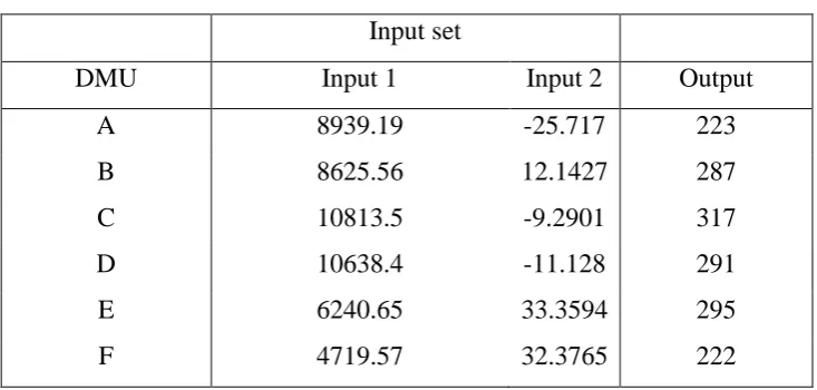
5.1. Example 1: To answer the question “who is best?” among six DMUs (Table 1), the Relocated
Input Oriented BCC DEA is applied. The efficiency is assessed from a conceived superior input reference point (0, -33.3) instead of (0, 0).
Table 1: Data
Input set
DMU
Input 1
Input 2
Output
A
8939.19
-25.717
223
B
8625.56
12.1427
287
C
10813.5
-9.2901
317
D
10638.4
-11.128
291
E
6240.65
33.3594
295
The outputs of the above model are shown in Table 2 and Table 3. From the theorems of DEA, it is well understood that B and D are truly inefficient (Table 2) whereas the rests need further tests for give assurance about their strongly efficient stature.
Table 2: RADIAL EFFICIENCY SCORE
Model
A
B
C
D
E
F
Transformed Model
1
0.93827
1
0.95371
1
1
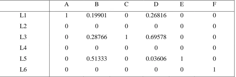
The coefficient matrix in Table 3 clarifies that B and D can be inferior DMUs than the corresponding hypothetical firms composed of A, C and E.Table 3: Values of Decision Variables
A
B
C
D
E
F
L1
1
0.19901
0
0.26816
0
0
L2
0
0
0
0
0
0
L3
0
0.28766
1
0.69578
0
0
L4
0
0
0
0
0
0
L5
0
0.51333
0
0.03606
1
0
L6
0
0
0
0
0
1
Apart from that B and D are not free from mix inefficiency (Table 4). Both of them do generate nonnegative input slacks in case of input 2. So, they remain inefficient in terms of both radial as well as mix measures.
Table 4: MEASUREMENT OF INPUT SLACKS
MODEL
Constraints
A
B
C
D
E
F
Translated
BCC Model
or
IO-RDM
INPUT 1
0
0
0
0
0
0
INPUT 2
0
2.05918
0
1.54409
0
0
OUTPUT
0
0
0
0
0
0
Output of the Rotated BCC DEA: The present problem has one input (input 1) which has all positive values. Thus, by keeping K1 as 50, the second constraint is transformed. The outputs of this model are shown in Table 5 and Table 6.
Table 5: RADIAL EFFICIENCY SCORE
MODEL
A
B
C
D
E
F
B and D both are found inefficient as before which are dominated by two hypothetical firms comprised with A, C and E.
Table 6: Values of Decision Variables
A
B
C
D
E
F
L1
1
0.1898
0
0.2596
0
0
L2
0
0
0
0
0
0
L3
0
0.25751
1
0.6677
0
0
L4
0
0
0
0
0
0
L5
0
0.55269
0
0.0727
1
0
L6
0
0
0
0
0
1
S1
0
0
0
0
0
0
R
0
0
0
0
0
0
Table 7: PREDICTION OF INPUT AND OUTPUT SLACKS (UNIT DEPENDENT)
MODEL
Constraints
A
B
C
D
E
F
TRANSFORMED
BCC DEA
INPUT 1
0
0
0
0
0
0
INPUT 2
0
0
0
0
0
0
OUTPUT
0
0
0
0
0
0
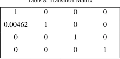
However, as expected the efficiency score of them are less as mentioned in Table 2. Apart from that there is no slack which gets a positive value (Table 7). Therefore, B and D no longer remain mix-inefficient.
The proposed model does have dual prices equal to or less than the original one (Theorem 3). However, the following transformation matrix can be engaged to derive one from the other.The dual price of the actual model can be derived from a matrix multiplication with a transposed dual price of the proposed model and the transition matrix (Table 8). The element in the second row and first column is set as
0.00462 (
𝐾1𝑎𝑜1
=
50 10813.5
).
Table 8: Transition Matrix
1
0
0
0
0.00462
1
0
0
0
0
1
0
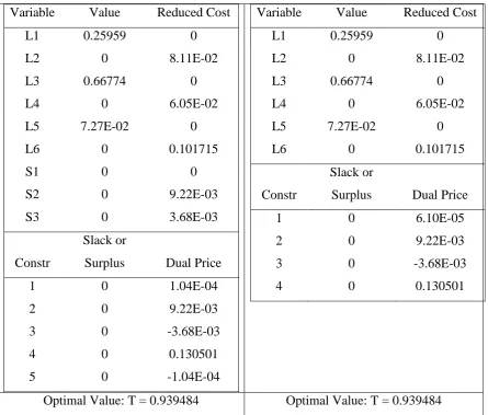
To test the effectiveness of the Transition Matrix , the performance of D is measured by using multiplier models on pre and post rotation data (Table 9). The optimal value and the values of decision variables remain same in both cases. However, a clear difference in the dual price can be observed in both cases. The original model has dual price greater than or equal to the proposed one. The matrix multiplication of the transpose of the dual price found in the proposed model with the transformation matrix will build up the dual price vector of the original model.
Table 9: Comparison of Outputs of Two Models
Variable
Value
Reduced Cost
L1
0.25959
0
L2
0
8.11E-02
L3
0.66774
0
L4
0
6.05E-02
L5
7.27E-02
0
L6
0
0.101715
S1
0
0
S2
0
9.22E-03
S3
0
3.68E-03
Constr
Slack or
Surplus
Dual Price
1
0
1.04E-04
2
0
9.22E-03
3
0
-3.68E-03
4
0
0.130501
5
0
-1.04E-04
Variable
Value
Reduced Cost
L1
0.25959
0
L2
0
8.11E-02
L3
0.66774
0
L4
0
6.05E-02
L5
7.27E-02
0
L6
0
0.101715
Constr
Slack or
Surplus
Dual Price
1
0
6.10E-05
2
0
9.22E-03
3
0
-3.68E-03
4
0
0.130501
Optimal Value: T = 0.939484
Optimal Value: T = 0.939484
Output of CCR DEA Model with and without rotation: To observe the effect of rotation on the results on the CCR model the two models, stated above, are run. Both models have astonishingly displayed the same results shown in Table 10 and Table 11.
Table 10: Radial Efficiency from CCR Models (with and without Rotation)
MODEL
A
B
C
D
E
F
The efficiency scores of B, C, D and F are indicative of radial inefficiencies which may be due to the presence of scale inefficiency (Table 10). All four DMUs referred before are being dominated by few hypothetical firms composed from the convex combination of A and E.
Table 11: Values of Decision Variables
A
B
C
D
E
F
L1
1
0.42033
0.87953
0.84582
0
0
L2
0
0
0
0
0
0
L3
0
0
0
0
0
0
L4
0
0
0
0
0
0
L5
0
0.65514
0.40971
0.34705
1
0.75254
L6
0
0
0
0
0
0
R
0
0
0
0
0
0
S1
0
0
0
0
0
0
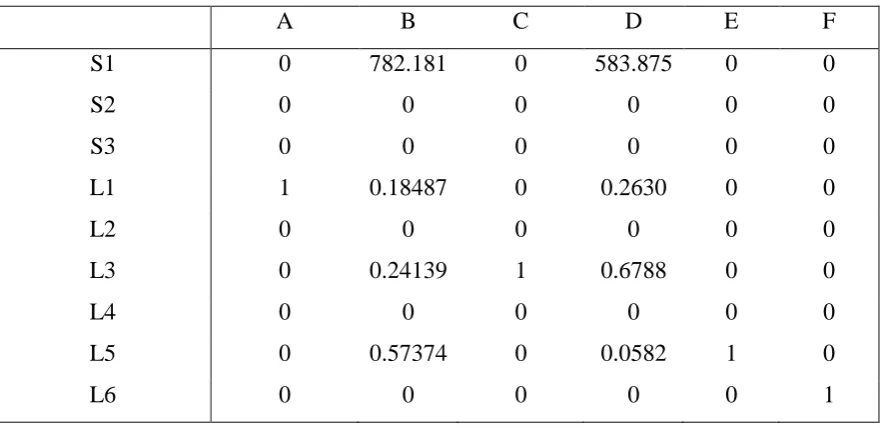
Output of SBM Model with and without rotation: Slack Based Additive model is referred for both occasions to verify the similarities of outcomes. Only one optimal table (Table 12) is mentioned here as the decision variables posses identical values on both the occasions. A and E are clearly efficient DMUs and others consume more than the required amount.
Table 12: Values of Decision Variables for Additive Model
A
B
C
D
E
F
S1
0
782.181
0
583.875
0
0
S2
0
0
0
0
0
0
S3
0
0
0
0
0
0
L1
1
0.18487
0
0.2630
0
0
L2
0
0
0
0
0
0
L3
0
0.24139
1
0.6788
0
0
L4
0
0
0
0
0
0
L5
0
0.57374
0
0.0582
1
0
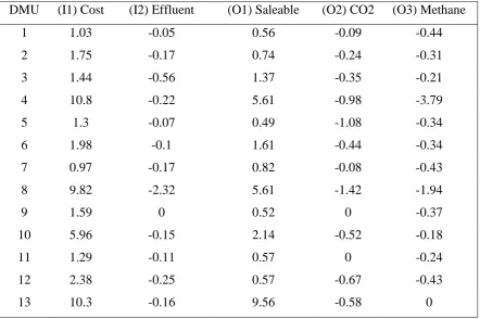
5.2. Example 2: The case of "notional Effluent Processing System" referred by Sharp et al (2006) is revisited here (Table 13).
Table 13: Notional effluent processing system
DMU
(I1) Cost
(I2) Effluent
(O1) Saleable
(O2) CO2 (O3) Methane
1
1.03
-0.05
0.56
-0.09
-0.44
2
1.75
-0.17
0.74
-0.24
-0.31
3
1.44
-0.56
1.37
-0.35
-0.21
4
10.8
-0.22
5.61
-0.98
-3.79
5
1.3
-0.07
0.49
-1.08
-0.34
6
1.98
-0.1
1.61
-0.44
-0.34
7
0.97
-0.17
0.82
-0.08
-0.43
8
9.82
-2.32
5.61
-1.42
-1.94
9
1.59
0
0.52
0
-0.37
10
5.96
-0.15
2.14
-0.52
-0.18
11
1.29
-0.11
0.57
0
-0.24
12
2.38
-0.25
0.57
-0.67
-0.43
13
10.3
-0.16
9.56
-0.58
0
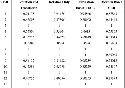
The problem referred here is a perfect example of partially negative data problem thus the proposed models can be approved here. Three variations are applied on the data set:
Rotation and Relocation Based Input Oriented BCC Model: The radial measure of efficiency is derived by offering rotation to the input side and adding an arbitrary value to the second output for translation. These treatments will allow the application of a regular BCC model.
Rotation Based Input Oriented BCC Model: Both input and output sides are transformed through the rotation process and a regular BCC model is applied afterwards.
Relocation Based Input Oriented BCC Model: Translation based model (which is similar to the IORDM+) is applied here.
Table 14: Output of the Proposed Models
DMU
Rotation and
Translation
Rotation Only
Translation
Based I BCC
Rotation Based
CCR
1
0.94175
0.94175
0.94566
0.57843
2
0.67505
0.67505
0.88102
0.44446
3
1
1
1
1
4
0.55804
0.55804
0.6613
0.55165
5
0.86275
0.86275
0.89149
0.39618
6
0.8584
0.8584
0.8584
0.85468
7
1
1
1
1
8
1
1
1
0.60065
9
0.81132
0.81132
0.95259
0.74015
10
0.45398
0.45398
0.83739
0.38167
11
1
1
1
1
12
0.40756
0.40756
0.80255
0.25173
13
1
1
1
1
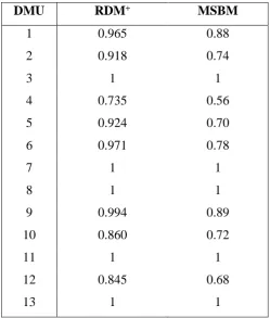
Assuming the existence of an Ideal Performer which consumes an input set of (0.97, -2.32) and produces an output set of (9.56, 0, 0) the RDM+ was applied on the data (Table 14). It is to be noticed that RDM+
provides Efficiency Score (which does not include any norm calculation) greater than or equal to IORDM+ (mentioned before). Since, RDM+ highlights the weakest area of performance in the context
of input consumption or output production, thus, the results of these two can only be same if the weakness exists on the Input side. However, inequality can also happen if output side is worse than the input side. A comparative study made in between Table 14 and Table 15 can reveal that each of these models are good enough to track the efficient DMUs. The author has verified that the results of MSBM (mentioned in Emrouznejad, A., Anouze, A. L. (2010) [5]) can also be regenerated from even after the application of rotation (while keeping the objective function same). Dissimilarities are largely observed in the outputs of MSBM and the proposed models because of an inequality of 𝜌𝑅𝐷𝑀≥ 𝜌𝐼𝑂𝑅𝐷𝑀 ≥ 𝜌𝑀𝑆𝐵𝑀. Following arguments can be cited to justify this statement. 𝜌𝑐,𝑀𝑆𝐵𝑀, being a MSBM efficiency
measure of any DMU-c, implicates all types of slack variables. Whereas, inefficiency in the model of IORDM (RDM) is (here 𝛽𝐼𝑐 (𝛽𝑐)) referred here to point out inefficiencies due to input handling (poor
performances in every possible arena of input and output set).
𝛽
𝐼𝑐= max (
𝑆𝐼𝑗𝑅𝐼𝑗
) 𝑎𝑛𝑑 𝛽
𝑐= max (
𝑆𝐼𝑗 𝑅𝐼𝑗
,
𝑆𝑂𝑗
𝜌
𝑐,𝑀𝑆𝐵𝑀=
1−1 𝑣∑
𝑆𝐼𝑖 𝑅𝐼𝑖 𝑣 𝑖=1
1+1
𝑚∑ 𝑆𝑂𝑗 𝑅𝑂𝑗 𝑚 𝑗=1
≤ (1 −
1𝑣
∑
𝑆𝐼𝑖
𝑅𝐼𝑖
𝑣
𝑖=1
) ≤ (1 −
𝑆𝐼𝑖′
𝑅𝐼𝑖′
) = 𝜌
𝐼𝑂𝑅𝐷𝑀≤ 𝜌
𝑅𝐷𝑀A rotation based CCR model is also applied to understand the extent of scale efficiency. DMU 5 faces the highest possible scale inefficiency whereas in spite of being almost scale efficient, DMU 4 and DMU 6 are inefficient due to their poor performances.
Table 15: Outputs of RDM and MSBM
DMU
RDM
+MSBM
1
0.965
0.88
2
0.918
0.74
3
1
1
4
0.735
0.56
5
0.924
0.70
6
0.971
0.78
7
1
1
8
1
1
9
0.994
0.89
10
0.860
0.72
11
1
1
12
0.845
0.68
13
1
1
6. Conclusion
In an example Portela et al (2004) [11] mentioned the problem of using negative data in a normal BCC DEA model which leads to improper radial directions and subsequently a different opinion from the slack based models. Shifting of origin to a superior or an inferior point is needed to make it eligible to identify the proper frontier. But, this method cannot generate unique outcome as the efficiency score can be better or worse due to the choice of such points. The first model, proposed here, counts everything from a new origin (which is superior to the old one). Any better choice than this new point will lead to enhancement of efficiency score. Moreover, like IO-RDM, this model is not translation invariant.
data is transformed into non-negative data. It can be seen from this small example that all these models are perfectly capable of identifying efficient and inefficient DMUs by determining efficiency scores accurately. Like the former model, the later one does not make an unnecessary interception on the frontier. But, in spite of the successful operation this model can never be applied if the condition stated before is violated. In a nutshell, if the input data does not have at least one member with all positive data then a relocation of origin will be the only way of getting solution. Lastly, from the example stated before it can be understood that a rotation process, unlike translation property, does not have reservations for any DEA models. It is therefore not at all necessary to relocate an Origin in case of a partially negative data and to score a better efficiency value due to it.
References
[1] Ali. A. I, Seiford. L. M., (1990) "Translation Invariance in Data Envelopment Analysis", Operations Research Letters: Vol-9, 403-405
[2] Banker, R. D., Charnes, A., Cooper, W. W. (1984). “Some models for estimating technical and scale inefficiencies in data envelopment analysis”. Management Science, 30(9), 1078-1092.
[3] Charnes, A., Cooper, W. W., & Rhodes, E. (1978). Measuring the efficiency of decision making units. European Journal of Operational Research, 2, 429-444.
[4] Cooper. W. W., Seiford. M. L., Tone. K., (2011)., Data Envelopment Analysis: A Comprehensive Text with Models, Applications, References and DEA-Solver Software, (2002), Kluwer Academic Publishers, New York, 2, 42-43.
[5] Emrouznejad, A., Anouze, A. L. (2010). “A semi-oriented radial measure for measuring the efficiency of decision making units with negative data, using DEA”. European Journal of Operational Research 200(1): 297-304.
[6] Farrell M. J. (1957), “The Measurement of Productive Efficiency”. Journal of Royal Statistical Society, Series-A: Vol-120: 253-281.
[7] Halme, M., Pro, T., Koivu, M., “Dealing with interval-scale data in data envelopment analysis”, European Journal of Operational Research, 137 (2002) 22-2.
[8] Matin, R. K, Azizi, R. (2010), “Modified semi-oriented Radial Measure for measuring the efficiency of DMUs”. With 3rd Operation, Research Conference.
[9] Pastor, J.T., (1993). “Efficiency of Bank Branches Through DEA: The Attracting of Liabilities”, Working Paper, Universidad de Alicante, Alicante, Spain.
[11] Portela. M. C. A. S, Thanassoulis. E and Simpson. G, (2004)., Negative data in DEA: a directional distance approachapplied to bank branches, Journal of the Operational Research Society. 55, 1111-1121
[12] Seiford L.M., (1989), A Bibliography of Data Envelopment Analysis, Working Paper, Dept Of Industrial Engineering And Operations Research, University Of Amherst, Ma 01003, USA.
[13] Sharp J. A., Lio W. B., Meng W., “A modified slack-based measure model for data envelopment analysis with “natural” negative outputs and input”, Journal of Operational Research Society, 57 (11) (2006) 1-6.
[14] Thrall R. M., (1996). “The lack of invariance of optimal dual solutions under translation”. Annals of Operations Research; 66: 103–108.