Third International Workshop on Vortex Flows and Related Numerical Methods
http://www.emath.fr/proc/Vol.7/
215
Viscous Flow Simulation of a Two-Dimensional Channel Flow with Complex
Geometry Using the Grid-Particle Vortex Method
Henryk Kudela
Wroclaw University of Technology 50-370 Wroclaw, Wybrzeze Wyspianskiego 27
e-mail: [email protected]
Abstract
To avoid a large consumption of computer time instead of the direct vortex methods with Biot-Savart interaction law, the vortex in cell method was used. The local velocity of a particle was obtained by the solution of the Poisson equation for the stream function, its differentiation, and then interpolation of velocity to the vortex particle position from the grid nodes. The Poisson equation for the stream function was solved by fast elliptic solvers. To be able to solve the Poisson equation in a region with a complex geometry, the capacitance matrix technique was used. The viscosity of the fluid was taken in a stochastic manner. A suitable stochastic differential equation was solved by the Huen method. The non-slip condition on the wall was realized by the generation of the vorticity. The program was tested by solving several flows in the channels with a different geometry and at a different Reynolds number. Here we present the testing results concerning the flow in a channel with sudden symmetric expansion.
1
Introduction
The vortex method has been used for the modelling of fluid dynamics phenomena for a long time. Rosenhead (1931) is regarded as the first person to use the point vortex for the numerical study of Kelvin -Helmholtz instability After him there were many other researchers who used the vortex elements and their ingenuity to study different fluid dynamics phenomena [12,13]. However only Chorin’s (1973) work relating to the simulation of viscous flow by the vortex blob method gave great impetus to the investigation and development of vortex methods. The algorithm was designed in such a way that the calculations were carried outs in Lagragian variables and was grid free. A viscous splitting algorithm was used. The solution was obtained in two steps. In the first step, the Euler equation was solved, in the second, the diffusion equation was solved. The local velocity of the blobs was calculated on the basis of the Biot-Savart law. That led to the direct summation of all the velocities induced by the vortex particles present in the flow. Due to the fact that, the number of operations in each time step is proportional to ∼0(N2
216 H. Kudela O(N+MlogM ) operation count (M being the number of points on the mesh) is less computationally intensive than the direct method based on the Biot-Savart law. One can find several papers where application of the VIC method is used successfully for the simulation of viscous flow [5, 26, 29].
The primary goal of the present work was the creation of a general purpose program for the solution of the viscous flow problem in a channel with a complex geometry on the basis of the VIC method.
2
Governing equations and a description of the vortex in cell method for
viscous flow
The non-dimensional equations of incompressible fluid motion in two-dimensional space transformed to the vorticity transport equations [8] take the form:
where • is the non-zero component of the vector vorticity, u = (u,v) is the velocity vector divided by the uniform inlet velocity U, • is the streamfunction, t - is the time and Re is the Reynolds number defined as Re=Uh/v where v is the coefficient of kinematic viscosity.
One can note that due to the incompressibility of the fluid,ΛΑu=0, equation (1) can be rewritten as:
Equation (3) is identical, with respect to the form, to the forward Kolmogorow -Fokker-Planck equation that describes the probability density called transition density for the stochastic Marcov process:[19];
where P is probability, G(x,t;• ,0) is a solution of equation (3). In the theory of the stochastic differential equation, it is shown that the stochastic process is described by a stochastic differential equation (in the Ito sense):
and it has the transition density that satisfies equation (3), where W means the Wiener process. So equation (5) describes the fluid motion in terms of stochastic processes. For the solution (5) we used a viscous splitting algorithm: velocity (drift) is calculated for inviscid flow (Euler equations) and the last term takes into account
)
3
(
Re
1
=
)
u
(
ω
ω
ω
∇
⋅
∆
∂
∂
+
t
)
2
(
x
-=
v
,
y
=
u
,
-=
∂
∂
∂
∂
∆
ψ
ω
ψ
ψ
)
1
(
1
=
)
u
(
ω
ω
ω
⋅
∇
∆
∂
∂
Re
+
t
)
4
(
x
)
0
,
(
)
)
(
(
X
t
A
,
t
=
G
x
,
t;
d
P
A
α
∫
∈
(5)
2
+
)
,
x
u(
)
X(
dW
Re
dt
the diffusion property of the fluid. In the present work, for the solution of equation (5) we use the generalized Huen scheme for the stochastic equations [19]:
(
)
W
t
Re
t
W
t
Re
t
n p n p p n p n p n n p n p2
+
)
x
(
u
x
x
where
)
6
(
2
)
x
(
u
)
(x
u
2
1
x
x
* * 1∆
∆
∆
+
=
∆
∆
+
∆
+
+
=
+where • Wn is an increment of the Wiener process, and • t is a time step. It is well known that the increments
of the Wiener process are the independent Gaussian random variables with mean E(• Wn )=0 and variance
E((• Wn)2)=• t; so it is relatively easy to generate it by a pseudo-random generator of numbers with uniform
distribution and using the Box-Muller transformation [19].
Now we will describe the VIC algorithm for obtaining the inviscid velocity field u(u,v). Vorticity • (x,y) is approximated by the linear combination of the Dirac measures:
where p is the number of the vortex particle. Approximation (7) is understood in the sense of measure on R2 [24]:
We assumed that we were able to solve the Poisson equation for the streamfunction (2) by the finite difference method. The computation goes as follows:
1) At first the redistribution of the mass of vortex particles on the grid nodes is done:
where νj(x)=ν((x-xj)/h), is a B-spline of order m [20]. For m = 1 the B-spline has the form:
and (9) is reduced to a well known area-weighted interpolation scheme [9]. In the present work we use the B-spline of the first order in the cells that adjoin the boundary of the domain flow, and outside these cells we used the B-spline of the 3rd order that takes the form [20,27]:
The B-splines satisfy: ν(x)=ν(-x) and Ιν(x)dx=1 [20,27]. To obtain the vorticity in the grid node, we should divide the circulation of the node obtained from (9) by the volume of the cell h2. Instead of that, Cottet [11]
)
7
(
)
x
(
),
x
(x
(x)
np p 2 n pp p n
h
ω
δ
ω
=
∑
Γ
−
Γ
=
)
8
(
)
(
)
(
2 ph
x
dx
x
∑
p∫
ω
≈
ω
)
9
(
)
(x
np pj p n
j
=
∑
Γ
Γ
ϕ
)
10
(
1
0
1
1
)
(
≤
>
|
x
|
for
|
x
|
for
|
x
|
=
x
ϕ
)
11
(
2
|
|
0
2
|
|
1
3
4
|
|
2
|
|
6
1
1
|
|
,
3
2
|
|
2
1
)
(
3 2218 H. Kudela
proposed, in order to overcome some difficulties related to the accumulation of the particles, the calculation of the volume of the nodes through the position of the particles around the node:
Then the vorticity in j node is calculated as:
2) We solved the Poisson equation for the streamfunction with a boundary condition that assured cancellation of the normal component of the velocity field on the wall (• =const, e.g • =0 and • =Q, where Q is a flow rate ):
)
14
(
ω
ψ −
=
∆
The velocity at the grid nodes is calculated by central difference:
)
15
(
2
)
,
(
)
,
(
2
)
,
(
)
,
(
2 1 2 1 2 1 2 1h
y
h
x
y
h
x
v
h
h
y
x
h
y
x
u
j j j j j j j j j j−
−
+
=
−
−
+
−
=
ψ
ψ
ψ
ψ
3) The value of the velocity from the grid nodes is interpolated to the position of the particles:
where lh is the base function of the Lagrangian interpolation. In the present work we took as lh(x) the B-spline
ν(x) of order one (m=1). This ends the computation process for VIC algorithm.
To satisfy the non-slip condition on the wall (Μ• /Μn=0) we utilized the vorticity generation process.
In numerical practice when the fluid equations are formulated in • -• terms one comes to the
problem of the determination of the vorticity value on the wall. In literature we can find a whole
family of different approximate formula allowing this to be done. One of the oldest and simplest
is the Thom`s formula [15,22]:
Formula (17) may by obtained from equation (14) when one writes it on the wall and takes into account that (• i,1-• i,-1)/(2• y
2
)=0 (index -1 is related to the “ghost” point outside the computational domain).
)
12
(
)
h
x
-x
(
h
=
)
x
(
h
=
J
2 j pp p j 2
p
j
∑
ϕ
∑
ϕ
)
13
(
)
x
(
h
x
=
J
=
p j 2 p p j p p j j j
)
(
ϕ
ϕ
ω
∑
∑
Γ
Γ
)
17
(
2
1 ,ψ
ω
B 2i
y
∆
−
=
)
16
(
)
x
(x
u
)
x
(
u
p p jAt each time step it is assumed that the formula (17) designates the proper amount of vorticity on the wall. If old vortex particles that already exist in the flow give to the boundary point by redistribution the vorticity • old then to the nodes point on the boundary is added the new portion of vorticity ωnew in such a way that:
The new portion of vorticity • new is redistributed among the nv vortex particles giving them the circulation
• =(• new h 2
)/nv where nv was chosen in such a way that |• |<0.05, (nv ε(2,11)).
A similar process of generation vorticity was successfully applied in papers [29, 5] . Instead of formula (17) the Woods formula [15,22] was also tested: • B = -3• 1/• y
2
-(1/2)• 1, where
• 1, • 1 correspond to the streamfunction and vorticity values at distance • y from the wall. The Woods
formula had the same order of accuracy and gave results similar to the Thom’s formula (17).
The final step in obtaining the solutions is the replacement of the vortex particles in accordance with formula (6) and the whole process begin in step 1).
For the solution of the Poisson equation a fast elliptic solver was used. To be able to solve the Poisson equation in an irregular region, the capacitance matrix technique was used. This technique is well described in many place in literature [3 ,23, 28].
3 Numerical
results
The program was tested for the flow in a channel with sudden, symmetric expansion (Fig.1). The length of the computational domain was taken as 32h where h=1 is the height of the step. The expansion ratio was Wo/W=1/3, or 0.5. The grid steps were taken as • x=• y=0.1, time step • t=0.01.
From literature it is known that together with the variation of the Reynolds number the flow undergoes several changes [1,4,14,16]. For a small Reynolds number, e.g Re=56 [4] the lengths of the
recirculation
zones
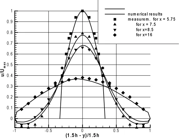
behind each step are equal and velocity profiles are symmetrical (Fig. 2). In Fig.3 we presented a comparison of calculated numerical results of velocity distribution at different cross sections along the channel with a measurement that was taken from the paper [14]. The agreement is good, but one may notices that the distribution of velocity near the wall is not as smooth as we had expected it to be.Growth of the Reynolds number causes the loss of symmetry (Re≈114). One of the recirculation zone becomes larger then the other. Further increasing the Reynolds number (Re≈252) causes that this greater recirculation zone breaks down into smaller one. All these phenomena one can see in Fig.4 where the streamlines for Reynolds number Re= 56, Re=125 and 252 were shown. It is in good qualitative agreement with results presented in literature [1,4 6 ].
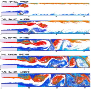
In Fig 5 we presented the sequence of the vortex particles position at Re=1000. One can see the formation of the eddies and again this is in good agreement with the picture published in [4] (see Fig.6).
)
18
(
ω
ω
220 H. Kudela We also carried out the calculation for the flow at a very high Reynolds number. The aim of these numerical experiments was to test the possibility of modelling the vorticity field evolution in flow at such a high Reynolds number by the VIC method described above. As it was pointed out by Chorin [7 ], one should keep in mind the difference between modelling with vortices and numerical approximations of solution of a fluid motion equation by the vortex method. It seems that the last experiment belongs to the “modelling”. This means we tried with the help of a moderate number of vortices to get qualitative understanding of the vorticity field dynamic at a very high Reynolds number. The sequence of the vortex particles for the flow at Re=105 is presented in Fig.7. It is easy to notice presence of vorticity filaments -- thread-like structures that are regarded as typical structures of two-dimensional turbulence [2,17,18,21]. One can observe that filaments are accompanied by a large coherent vortex structure that stabilizes them [18]. These large vortex structure are build with the both sings of vortex particles. Vortices of the same sign may undergo merging and vortices of opposite sign may form dipoles [18, 21]. All these mentioned phenomena we may find in the description of two dimensional turbulence in literature [17,21].
4
Conclusion
It seems that now it is not far from the creation of a general flow simulation package based on the vortex method into which the user need only enter minimal data concerning boundaries in order to be able to perform the numerical investigations. The present paper is a move in that direction. Vortex methods provide natural, useful tools for analysing flow in term of vorticity dynamics, and the visualization of the flow by vortex particles. The study of the evolution of the vorticity field helps one to understand the features of flow in a complicated geometry. It is one of the few methods which give reasonable results at large interval of Reynolds numbers. Further studies on the vortex method, e.g. on cancellation of tangential velocity on the wall, on the simulation of diffusion, and on the redistribution of circulation particles to the grid nodes in the VIC method should, it is believed improve the numerical results.
References
[1] Allebron N., Nandakumar K.,Raszillier H., Durst F.: Further contributions on the two-dimensional flow in sudden expansion , J.Fluid Mech.,1997 v.330, (1997) pp. 169-188.
[2] Brachet M..E., Meneguzzi M., Politano H., Sulem P..L.:The dynamics of freely decaying two-dimensional turbulence, vol. 194, (1988), pp. 333-349.
[3] Buzbee B. L., Dorr F.W.,George J. A., Golub G. H.: The solution of the discrete Poisson equation on irregular regions, SIAM, J. Num. Anal., vol. 8, (1971), pp. 722-736.
[4] Cherdron W., Durst F., Whitelaw J.H.: Asymmetric flows and instabilities in symmetric ducts with sudden expansions, J.Fluid Mech., vol. 84, (1978), pp. 13-31.
[5] Chang C. C., Chern R.-L.: A numerical study of flow around an impulsively started circular cylinder by a deterministic vortex method, J. Fluid Mech., vol. 233, (1994), pp. 243-263.
http://www.emath.fr/proc/Vol.1/contents.htm
[8] Chorin A.J., Marsden J.E.: A Mathematical Introduction to Fluid Mechanics, Springer 1979.
[9] Christiansen J.P.: Numerical simulation of Hydrodynamics by the Method of Point Vortices, J.1 Comp. Phys., Vol. 13 (1973), pp. 363-379.
[10] Cottet G-H.: Convergence of a vortex in cell-method for the two-dimensional Euler Equations, Math. Comput. Vol.49, (1987), pp.407-420.
[11] Cottet G-H. A A particle-grid superposition method for the Navier-Stokes equations, J. Comp.. Phys., (1980), vol. 89, pp. 301-318.
[12] Clements R.R : Flow representation, including separated regions, using discrete vortices, Lecture Series no. 86., on Computational Fluid Dynamics, AGARD, (1976), ss.5/1-5/20
[13] Clements R.R, Maull D.J: The representation of the sheets of vorticity by discrete vortices, Porg. Aerospace Sci., vol. 16, no.2, (1975), p.129
[14] Durst F., Melling A., Whitelaw J.H.: Low Reynolds number flow over a plane symmetric sudden expansion, J,Fluid Mech, 1974, vol. 64, pp. 111-128.
[15] E Weinan, Liu Jian-Guo: Vorticity boundary condition and related issues for finite difference schemes, J. Comput. Phys 1996, vol 124, pp. 368-382
[16] Faren R.M., Mullin T., Cliffe K.A.: Nonlinear flow phenomena in a symmetric sudden expansion, J.Fluid Mech., 1990, vol. 124, pp. 368-382
[17] McWilliams J.C.:The emergence of isolated coherent vortices in turbulent flow, J. Fluid Mech. 1984, vol. 146, pp.21-46.
[18] Kevlahan N. K.-R. Farge M.: Vorticity filaments in two-dimensional turbulence: creation, stability and effect, J. Fluid Mech (1997), vol. 346, pp. 49-76
[19] Kloeden P., Platen E.: Numerical Solution of Stochastic Differential Equations, Springer, 1982 [20] Kong J. X., Contribution a l'analyse numericque des methodes de couplage particules-grille en mecanique
des fluides, Phd. dissert., Universite J. Fourier Grenoble, LMC-IMAG 1993. [21] Lesieur M., Turbulence in Fluids, Third edition, Kluwer Academic Publishers, 1997 [22] Peyret R., Taylor T. D.: Computational methods for fluid flow, Springer-Verlag (1983)
[23] Proskurowski W., Widlund O.: On the numerical solution of Helmholtz’s equation by the capacitance matrix method, Math. Comput., vol.30, ,(1976), s.433-468
[24] Raviart P...A.: An analysis of particle methods, in Numerical methods in fluid Dynamics , ed. Brezzi F., Lecture Nots in Mathematics, vol. 1127, (1985) ss. 243-324, Spinger Verlag, Berlin
[25] Rosenhead L.: The formation of vortices from a surface of discontinuity, Proc. R. Soc. Lond., A 134, (1931), ss. 170 -192.
[26] Savoie R., Gagnon Y.: Numerical Simulation of the Starting Flow Down a Step, ESAIM: Proceedings, Vortex Flows and Related Numerical Methods II, 96, Vol. 1, 1996, pp. 377-386, http://www.emath.fr/proc/Vol.1/contents.htm
[27] Schoenberg I.J.: Contributions to the problem of approximation of equidistant data by analytic function, Part A, Quart. Appl. Math. 1946, vol. 4. pp. 45-99.
[28] Schumann U., Sweet R.A.: Direct Poisson Equation Solver for Potential and Pressure Fields on a Staggered Grid with Obstacles, Lecture Notes in Physics, vol.59, (1976), pp. 397-403.
222 H. Kudela
\
[ K
: :
8
Fig. 1 The sketch of the geometry for the flow over a plane symmetric sudden expansion
Fig.2 Averaged streamlines with the velocity profiles at Re=56, Wo/W1/3, Wo=h
Fig. 3. Comparison of the numerical results with measurements taken from [14].
K \ K
X
8PD
[
QXP H ULFD O UH VXOWV P H D VXUH P IRU [
Fig.4 The field of streamfunction values with streamlines at Re=56,Re=125, R=252, Wo/W=1/3.
Fig 5. The sequence of vortex particle positions at Re=1000, Wo/W=1/2..
7 5 H 1
7 5 H 1
224 H. Kudela
Fig. 6 Scanned picture of the experimental visualization from the paper [4] (Fig.9d, Re=800.)
![Fig. 6 Scanned picture of the experimental visualization from the paper [4] (Fig.9d, Re=800.)](https://thumb-us.123doks.com/thumbv2/123dok_us/10091219.1995812/10.595.116.487.213.594/fig-scanned-picture-experimental-visualization-paper-fig-d.webp)
