A new approach for data visualization problem
MohammadRezaKeyvanpour ,Mona Soleymanpour
Received (2015-08-09) Accepted (2015-10-18)
Abstract — Data visualization is the process of transforming data, information, and knowledge into visual form, making use of humans’ natural visual capabilities which reveals relationships in data sets that are not evident from the raw data, by using mathematical techniques to reduce the number of dimensions in the data set while preserving the relevant inherent properties. In this paper, we formulated data visualization as a Quadric Assignment Problem (QAP), and then
presented an Artificial Bee Colony (ABC) to
solve the resulted discrete optimization problem. The idea behind this approach is to provide
mechanisms based on ABC to overcome trapped
in local minima and improving the resulted
solutions. To demonstrate the application of ABC
on discrete optimization in data visualization, we used a database of electricity load and compared the results to other popular methods such as SOM, MDS and Sammon’s map. The results show that
QAP-ABC has high performance with compared
others.
Keywords - Data visualization, Quadric
Assignment Problem (QAP), Artificial Bee Colony (ABC)
I. INTRODUCTION
D
ata visualization is a graphical presentation of multidimensional data making use of humans’ natural visual capabilities.More specifically, data visualization reveals
relationships in data sets that are not evident from the raw data, by using mathematical techniques to reduce the number of dimensions in the data set while preserving the relevant inherent properties. Compared with the data appear in their original high dimensional space, we may be more capable
of finding the possible relationship among the
data points in the low dimensional space, i.e., 2-D. therefore, it has been widely applied to solve many problems, e.g. signal compression, pattern recognition, image processing, etc[1].
Dimensionality reduction or projection techniques can transform large data of multiple dimensions into a smaller, more manageable set with special methods. Principal component analysis (PCA) and MultiDimensional Scaling (MDS) are two popular methods for data reduction and visualization. PCA is one of the
most widely used methods because it is effective
and robust for performing linear projection. Linear projection means the projection of data is conducted by multiplying each component of the original vector with a scalar. Thus, PCA is not the most suitable approach when one is dealing with highly nonlinear data. MDS is another
classical projection but its final visualization map is difficult to perceive, when one is handling
high dimensional and highly unsymmetrical data set. Sammon’s mapping is the earliest approach in nonlinear projecting data into low dimensional space for visualizing multivariate data. Sammon’s mapping tries to minimize the
1- Department of Computer Engineering, Alzahra University, Tehran, Iran ([email protected])
distances between input data in the original high dimensional space and the output data in the projected space. It is capable of preserving the topological structure of the original data and their corresponding inter point distances, but Sammon’s mapping is computationally demanding especially when one is handling huge numbers of data points. Inaddition, itrequiresre-computationwhennewdatapoints are added[2, 3]. Discrete optimization techniques provide a possible alternative for the data visualization problem. Discretizing the data visualization problem may result in a large-scale quadratic
assignment problem that is very difficult to solve
to optimality [4]. The complexities of these problems are high and it is a NP Complete. One approach to overcome high large-scale quadratic assignment and its complexity is solving it by heuristics or intelligent optimization.As more and more real-world optimization problems become increasingly complex, algorithms with more capable optimizations are also increasing in demand. We formulate the data visualization problem as a Quadric Assignment Problem
(QAP) and then use theArtificial Bee Colony
(ABC) to solve it.The idea behind this approach is to provide mechanisms based on ABC to overcome trapped in local minima and improving the resulted solutions.To evaluate our method we use a real data set and compare our proposed hybridapproach which is named QAP-ABC with SOM, MDS and Sammon’s Map as popular methods for data visualization.
The rest of the paper is organized as follows. Section 2 reviews relevant works in data visualization. Section 3 introduces modeling the problem as a Quadratic Assignment Problem
anddiscusses Artificial Bee Colony (ABC) to
solve this problem in detail. Section 4 presents a case study to evaluate the technique with experimental results, and then compares it with Self-Organizing Maps (SOM), Sammon’s Map (SM) and MultiDimensional Scaling (MDS) in section 5. Section 6 concludes the paper.
II. Background
The most common data visualization methods allocate a representation for each data point in a lower-dimensional space and try to optimize these representations so that the distances between them are as similar as possible to the original distances of the corresponding data items. The
methods differ in that how the different distances
are weighted and how the representations are optimized. Linear mapping, like principle
component analysis, is effective but cannot truly reflect the data structure. Non-linear mapping,
like Sammon’s Mapping(SM), MultiDimensional Scaling (MDS) and Self-Organizing Map (SOM) [5, 6], requires more computation but is better at preserving the data structure.
1. Sammon’s Mapping (SM)
Sammon Jr. [7]introduced a method for nonlinear mapping of multidimensional data into a two- or three-dimensional space. This nonlinear mapping is a MultiDimensional Scaling (MDS) projection which preserves approximately the inherent structure of the data and thus is widely used in pattern recognition. It tries to match the pairwise distances in the lower-dimensional representations with their original distances [3].
Denote the data vector 𝑥𝑥𝑖𝑖ൌ 𝑥𝑥𝑖𝑖ͳǡ𝑥𝑥𝑖𝑖ʹǡ…ǡ𝑥𝑥𝑖𝑖𝑑𝑑 𝑇𝑇ǡ 𝑖𝑖ൌ ͳǡ…ǡ𝑁𝑁 (N is the
number of data points) in a d-dimensional input space and the corresponding vector
𝑦𝑦𝑖𝑖ൌ 𝑦𝑦𝑖𝑖ͳǡ𝑦𝑦𝑖𝑖ʹǡ…ǡ𝑦𝑦𝑖𝑖𝑑𝑑 𝑇𝑇 in a l-dimensional out-put
space(l=2or3). Define the distance between xi
and xj in the input space as 𝑑𝑑𝑖𝑖𝑗𝑗∗ ≡ 𝑑𝑑 𝑥𝑥𝑖𝑖ǡ𝑥𝑥𝑗𝑗 and
the distance betweeny_i and yj in the output space as 𝑑𝑑𝑖𝑖𝑗𝑗 ≡ 𝑑𝑑 𝑦𝑦𝑖𝑖ǡ𝑦𝑦𝑗𝑗 . Distances are measured by
Euclidian metric. Error E is defined as follows:
𝐸𝐸 ൌ ͳ
𝑑𝑑𝑁𝑁 𝑖𝑖𝑗𝑗∗ 𝑖𝑖൏𝑗𝑗
𝑑𝑑𝑖𝑖𝑗𝑗∗ − 𝑑𝑑𝑖𝑖𝑗𝑗 ʹ
𝑑𝑑𝑖𝑖𝑗𝑗∗ 𝑁𝑁
𝑖𝑖൏𝑗𝑗
(1)
fast computers, nonlinear optimization techniques
are usually slow and inefficient for large data
sets. In addition,sincetheerrorisminimizedbythest eepestdescent procedure,itiseasilytrappedinlocal minima[2, 3, 8].
2. MultiDimensional Scaling (MDS)
Multidimensional Scaling (MDS) refers to a class of algorithms that visualize proximity relations of objects by distances between points in a low-dimensional Euclidean space. MDS algorithms are commonly used to visualize proximity data (i.e., pairwise dissimilarity values instead of feature vectors) by a set of representation points in a suitable embedding space[9, 10].
Let D={x1,x2,…,xn} be a set of nobjects in a d-dimensional feature space, and let dis denote the Euclidean distance between xi and xs. Let d*
be the number of dimensions of the output space,
xi* be a d*-dimensional point representing xi in the output space, and dis* denote the Euclidean distance between xi* and xj* in the output space. Let X be an n × d-dimensional vector denoting the coordinates xij (1≤i≤n , 1≤j≤d) as follows:
𝑥𝑥𝑖𝑖 ൌ 𝑥𝑥ͳǡ𝑥𝑥ʹǡ…ǡ𝑥𝑥𝑛𝑛𝑑𝑑 𝑇𝑇ǡ (2)
Where x(i-1)d+j= xij for i=1,2,…,n and j=1,2,....,d
Error EMDS is defined as follows:
𝐸𝐸𝑀𝑀𝐷𝐷𝑆𝑆 ൌ 𝑑𝑑𝑖𝑖𝑠𝑠
∗ − 𝑑𝑑
𝑖𝑖𝑠𝑠 ʹ
ͳ≤𝑖𝑖≤𝑠𝑠≤𝑛𝑛
𝑑𝑑𝑖𝑖𝑠𝑠ʹ
ͳ≤𝑖𝑖≤𝑠𝑠≤𝑛𝑛
(3)
The only difference between Sammon’s
Mapping and the nonlinear metric MDS is that (excluding the constant normalizing factor) the errors in distance preservation are normalized by the distance in the original space. Due to normalization, the preservation of small distances will be emphasized [9, 11].
The minimization of Error EMDS is a
optimization problem which is non-convex and sensitive to local minima and the main limitation of most MDS applications is that it requires O(N2) memory as well as O(N2) computation [12]. Thus, though it is possible to run them with small data size without any trouble, it is impossible to execute them with a large number of data due to memory limitation; therefore, this challenge could be considered as being a memory-bound
problem. Moreover, the MDS final visualization
map is difficult to perceive, when one is handling
high-dimensional and highly unsymmetrical data set [1, 13].
3. Self-Organizing Maps (SOM)
SOM, proposed by Kohonen[14], is a class of neural networks trained in an unsupervised manner, using competitive learning. It is a well-known method for mapping a high-dimensional space onto a low-dimensional one. It is popular to consider mapping onto a two-dimensional grid of neurons. The method allows putting complex data into order, based on their similarity, and shows a map by which the features of the data can be
identified and evaluated. A variety of realizations
of SOM has been developed [5, 6].
The SOM architecture consists of two fully
connected layers: an input layer and a Kohonen
layer. Neurons in the Kohonen layer are arranged in a one- or two-dimensional lattice. Fig. 1 displays the layout of a one-dimensional map where the output neurons are arranged in a one-dimensional lattice. The number of neurons in the input layer matches the number of attributes of the objects. In the input layer each neuron has a feed-forward connection to each neuron in the Kohonen layer [3].
Inputs (x) Weights
(w) Input layer
Output layer
M
1 2 m
x 1
x 2
x n
1 2 n
w n m w
1 1
Fig. 1.The structure of Self-Organization Map (SOM)
III. Data Visualization Problem: Definition and
Formulation
Discrete optimization techniques provide a possible alternative for the data visualization problem. Discretizing the data visualization problem may result in a large-scale Quadratic
Assignment Problem that is very difficult to
solve. Roselyn Abbiw-Jackson [4] used the divide and conquer algorithm to solve the Quadratic Assignment Problem (QAP). We concentrate solve data visualization problem as discrete optimization.
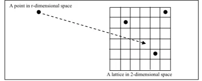
A point in r-dimensional space
A lattice in 2-dimensional space
Fig. 2. Structure of discretizing the data visualization problem
Let M be a set with n points in r-dimensional space (Rr). The data visualization problem
is locating any r-dimensional point in M to
q-dimensional space (Rq , q<r and q=2 or
3) such that a relevant measure of distance is preserved (Fig. 2). We use discrete optimization techniques to solve it. Therefore, we approximate the continuous q-dimensional space by a lattice
N while each cell has a center point. On the other hand, the data visualization problem is similar to assigning m point to n cell (center) points. The
decision variables are given by:
xik=�1, if thei
𝑡𝑡𝑡𝑡ℎinstance is assigned to lattice point k∈N
0, Otherwise
(4)
Therefore, data visualization problem can be
written as follows:
ǡǡǡ
𝑛𝑛
𝑙𝑙ൌͳ
𝑛𝑛
𝑘𝑘ൌͳ
𝑗𝑗ൌͳ
𝑗𝑗𝑖𝑖
ൌͳ
subject to ൌͳǡ∀ ∈
∈
xik∈ 0,1,
(5)
Where, 𝐷𝐷𝑜𝑜𝑙𝑙𝑑𝑑 ∈ 𝑅𝑅𝑚𝑚 ൈ𝑅𝑅𝑟𝑟 is a matrix
measuring the distance between n given instances,
∈ൈ is a new distance matrix
between assigned instances in the q=2 or 3 dimensional space and F is a function of the
deviation between the differences between the
instances in the original space and the new
q-dimensional space. Choices for F include the functions for Sammon’s Mapping and classical scaling, and all objective functions for non-metric scaling. By using Sammon’s Mapping as objective function, data visualization problem
can be formulated as:
ͳ ǡ ൌͳ
ൌͳ
ሺǡ Ǧȗǡ ሻʹ
ǡ
ൌͳ
ൌͳ
ൌͳ
ൌͳ
subject to ൌͳǡ∀ ∈
ൌͳ
xik∈ {0,1}ǡ
(6)
(6)
Where, d(i,j) is distance (usually Euclidean distance) between original points in space of Rr
and d*(k,l) is distance between lattice points in space of Rq.
The number of cells is determined with regards to requirement of data visualization method. A problem with points spread out will require a larger grid than one with points clustered together. The larger the grid, the more
accurate the final result. To scale the cells (in q-dimensional space) and the given data set,
we find the greatest distance between the pairs
of points in given data set. Let this distance be a and the greatest distance in the chosen lattice
problem is very large and decision variables are internally depended.
Any solution method can be used to solve
this problem but it should be effective in
circumstance of problem. Proposed solution
method here is Artificial Bee Colony named
QAP-ABC for solving data visualization problem as a discrete optimizationproblem. The idea behind this approach is to provide mechanisms for improving the data visualization precise. To introduce the proposed method, it is necessary
to give a brief review of Artificial Bee Colony
andits framework.
III. Proposed Method: QAP-ABC
The Artificial Bee Colony (ABC) method is
inspired by the intelligent foraging behavior of a honey bee colony in which bees try to maximize the nectar amount loaded into the hive by bees
assigned a specific task. In the foraging behavior,
there are three types ofbees, each of which has a
different search characteristic: these are employed
bees, onlooker bees and scout bees. The employed bees are responsible for exploiting the sources in their memory whereas the onlooker bees go to exploit potentially rich sources depending on the information taken by communicating with the employed bees. Scout bees are responsible for exploring undiscovered sources by a random motivation or external clue[15, 16].
The ABC algorithm mimics this foraging behavior of honey bees in the context of a global optimization algorithm. From the perspective of a meta-heuristic, a population of solutions corresponds to the food sources to be discovered
and the optimization task is to find the most profitable source by using the different search
characteristics of the employed bees, onlooker bees and scout bees[17-19]. Each type of bee is a phase of the algorithm as given in Fig. 3.
The perturbation strategy in ABC approach by using of calculation of 𝑥𝑥𝑥𝑥𝑖𝑖𝑖𝑖𝑖𝑖𝑖𝑖′ provides the solution
to move towards promising regions of the search space. This is the positive feedback of the ABC algorithm. By a greedy selection in step7, the new solution is kept in the memory and the current one is discarded if the new solution is better; otherwise, it is discarded, and the current one is retained in the population and a counter associated with the current solution is incremented
by one in order to count the number of nonprogressive local searches in the neighborhood of the current solution. This counter will be used to determine the exhausted sources to be used in the phase for scout bees. In the phase for employed bees, the local searches are conducted for all solutions in turn, while in the phase for onlooker bees they are carried out for the solutions chosen probabilistically. This probabilistic selection provokes high quality solutions to be chosen more, but also allows poor solutions to be selected. This selection scheme is also another positive feedback of the ABC algorithm [17, 20]. It is clear from the above explanation that there
are three control parameters in the basic ABC:
The number of food sources which is equal to the number of employed or onlooker bees (SN), the value of dimension of the problem (D) and the maximum cycle number (MCN).
In our proposed approach (QAP-ABC), we transform the data visualization problem to a Quadratic Assignment Problem (QAP) and apply ABC algorithm to optimize it. Then use the best
bee in final phase of ABC algorithm for projection
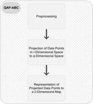
of original data points to a map and providing the output lattice.The Block Diagram of QAP-ABC is presented in Fig. 4.
As it is seen in Fig. 4, our proposed approach has three phases which detailed explained in
fallows:
1. Preprocessing
Since it is possible that the used data set has been comprised missed, inconsistence or noisy data, thus it is required to improve the quality of the actual data for mining by data pre processing. This
also increases the mining efficiency by reducing
the time required for mining the preprocessed data. Data preprocessing involves data cleaning, data integration, data transformation, data reduction, data normalization and etc. this phase is done same approach in[21].
2. Projection of Data Points in r-Dimensional Space to q-Dimensional Space
Before introducing the ABC algorithm, it is necessary to give used notation in this algorithm. Let, k: A uniform random index from [1,𝐶𝐶𝐶𝐶𝐶𝐶𝐶𝐶]interval and it has to different from 𝑖𝑖𝑖𝑖.
CS: The number of food sources.
j: The uniform random index that is belong to [1,𝐷𝐷𝐷𝐷]. D: The dimension of the problem.
fitnessi: The fitness value of the solution i. 1: Initialize the population of solution 𝑥𝑥𝑥𝑥𝑖𝑖𝑖𝑖𝑖𝑖𝑖𝑖
𝑥𝑥𝑥𝑥𝑖𝑖𝑖𝑖𝑖𝑖𝑖𝑖 =𝑥𝑥𝑥𝑥𝑖𝑖𝑖𝑖𝑚𝑚𝑚𝑚𝑖𝑖𝑖𝑖𝑚𝑚𝑚𝑚+ rand(0, 1)�𝑥𝑥𝑥𝑥𝑖𝑖𝑖𝑖𝑚𝑚𝑚𝑚𝑚𝑚𝑚𝑚𝑥𝑥𝑥𝑥 −𝑥𝑥𝑥𝑥𝑖𝑖𝑖𝑖𝑚𝑚𝑚𝑚𝑖𝑖𝑖𝑖𝑚𝑚𝑚𝑚� (7)
2: Evaluate the population 3: Cycle = 1
4: Repeat
5: Produce new solution𝑥𝑥𝑥𝑥𝑖𝑖𝑖𝑖𝑖𝑖𝑖𝑖′ for the employed bees using fallowing equation:
𝑥𝑥𝑥𝑥𝑖𝑖𝑖𝑖𝑖𝑖𝑖𝑖′ =𝑥𝑥𝑥𝑥𝑖𝑖𝑖𝑖𝑖𝑖𝑖𝑖+∅𝑖𝑖𝑖𝑖𝑖𝑖𝑖𝑖 �𝑥𝑥𝑥𝑥𝑖𝑖𝑖𝑖𝑖𝑖𝑖𝑖− 𝑥𝑥𝑥𝑥𝑘𝑘𝑘𝑘𝑖𝑖𝑖𝑖� (8)
6: Evaluate the population
7: Apply the greedy selection process between 𝑥𝑥𝑥𝑥𝑖𝑖𝑖𝑖𝑖𝑖𝑖𝑖 and 𝑥𝑥𝑥𝑥𝑖𝑖𝑖𝑖𝑖𝑖𝑖𝑖′ 8: Calculate the probability values 𝑝𝑝𝑝𝑝𝑖𝑖𝑖𝑖as follows:
𝑝𝑝𝑝𝑝𝑖𝑖𝑖𝑖=∑𝐶𝐶𝐶𝐶𝐶𝐶𝐶𝐶𝑓𝑓𝑓𝑓𝑖𝑖𝑖𝑖𝑓𝑓𝑓𝑓𝑚𝑚𝑚𝑚𝑓𝑓𝑓𝑓𝑓𝑓𝑓𝑓𝑓𝑓𝑓𝑓𝑖𝑖𝑖𝑖𝑓𝑓𝑓𝑓𝑖𝑖𝑖𝑖𝑓𝑓𝑓𝑓𝑚𝑚𝑚𝑚𝑓𝑓𝑓𝑓𝑓𝑓𝑓𝑓𝑓𝑓𝑓𝑓𝑖𝑖𝑖𝑖
𝑖𝑖𝑖𝑖=1 (9)
9: Produce new solution 𝑥𝑥𝑥𝑥𝑖𝑖𝑖𝑖𝑖𝑖𝑖𝑖′ for the onlookers depending on pi 10: Evaluate the population
11: Apply the greedy selection process between 𝑥𝑥𝑥𝑥𝑖𝑖𝑖𝑖𝑖𝑖𝑖𝑖and 𝑥𝑥𝑥𝑥𝑖𝑖𝑖𝑖𝑖𝑖𝑖𝑖′
12: Determine the abandoned solution, if exists, and replace it with a new randomly produced solution 𝑥𝑥𝑥𝑥𝑖𝑖𝑖𝑖for the scout. 13: Memorize the best food source position achieved so far
14: Cycle = Cycle + 1
15: Until Cycle = Maximum Cycle Number or time = Maximum CPU time
Fig. 3. Pseudo code of the basic ABC algorithm
QAP-ABC
Projection of Data Points inr-Dimensional Space toq-Dimensional Space
Preprocessing
Representation of Projected Data Points to
a 2-Dimensiond Map
Fig. 4. Block Diagram of QAP-ABC
Artificial Bee Colony
Apply the greedy selection process for recruit the onlooker bees to search around scout bees Data set
The output lattice Cycle < MCN Yes
No
Initialize the population of employed bees
Calculate the fitness value of each employed bee respectively
Select the scout bees using the roulette wheel selection operator
Searching nectar source just around the solution space
Reinitialize the population of employed bees
Keep the best solution parameters and the best fitness value
Using the best solution for providing of 2-dimentional map Preprocessing
Cycle = Cycle + 1 Cycle=1
data points. We concentrate to this phase in our
article.The flowchart of our proposed approach to
solve data visualization problem using of ABC algorithm is presented in Fig. 5.
3. Representation of Projected Data points to a 2-Dimensiond Map
We use the best bee resulted from ABC to project the high dimensional data points in r-dimensions to 2-dimensionals (q=2) space. As it is presented in Fig. 6, the best bee has 366*2=732 cells that ith pair of cells corresponds to the coordinate of ith original data points in output map which
i=1,2,3,…,366. The best resulted solution from ABC has minimum error, thus it guaranty to preserving the structure of the relationships between original data points in output map.
y366 x366 y365 x365
…
y2 x2 y1 x1
Best Solution
(x1,y1) (x2,y2) (x365,y365) (x366,y366)
Fig. 6.The best solution resulted from ABC representation
IV. Experimental Results
This section evaluates the performance of the QAP-ABC, SOM, MDS and Sammon’s Map to data visualization. Experiments were performed using an Intel Core 2 Duo, 2.1 GHz processor with 2 GB of RAM.
1. Data Set
In order to compare the proposed technique (QAP-ABC) and the well-known methods such as Self-Organizing Maps algorithm (SOM), Sammon’ Map and MDS,a real-life case is considered here. Used data set in this research includes 24-hour electrical load of 366 days starting from 20 March 2008 in Esfahan. Therefore, we have 366 instances with 24 attributes, which any attribute is as an hour (a label number for all the daily load curves).
2. Parameters Setting
The dimension of the output map in this research is assumed to be two (q=2), because
most visible media (for example: paper, monitor
panel and etc.) are 2-dimensional. The output
map is a 60×60 grid square. Dimension of the output map is calculated by a heuristic function in SOM toolbox in MATLAB [22].
ABC settings:Except common parameter
(maximum cycle number), the basic ABC used in this study employs two control parameters D and SN. The maximum cycle number is supposed 2000 and other ABC parameters is resulted from
[18] as: In original ABC algorithm, 50% of the colony consists of employed and the rest 50%
consists of onlooker bees. In other words, the ratio of employed and onlooker bees are the
same, 1:1 [23]. Therefore, we use ratio 1:1 in
this study. To reach the optimal parameters we
run ABC with different parametersD and SN. The
ABC program was run 30 times and average of observations register for any parameters. Table1
and Fig.7show the results of original (ratio 1:1) ABC algorithms with different D and SN.
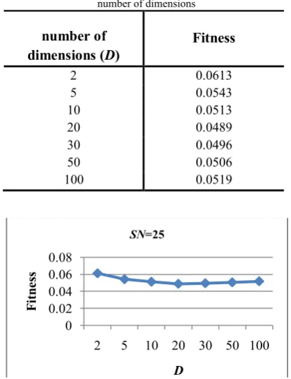
Table 1. Fitness values for QAP-ABC with SN=25 and various number of dimensions
number of
dimensions (D) Fitness
2 0.0613
5 0.0543
10 0.0513
20 0.0489
30 0.0496
50 0.0506
100 0.0519
0 0.02 0.04 0.06 0.08
2 5 10 20 30 50 100
Fi
tne
ss
D
SN=25
Fig. 7. The sensitivity of ABC to number of dimensions (D) in QAP-ABC
The result of QAP-ABC with SN=25 and various number of dimensions (D) is shown in Fig.7 and Table.1. As it is shown in Fig.7 and Table1 more number of dimensions improves the
fitness. The decreasing of fitness by increasing
D=20 and different SN (see Table 2 and Fig. 8).
Table2. Fitness values for QAP-ABC with D=20 and various number of onlooker bees
Onlooker Bees (SN) Employed bees Fitness
10 10 0.0541
25 25 0.0489
50 50 0.0439
75 75 0.0395
100 100 0.0351
125 125 0.0332
150 150 0.0327
175 175 0.0327
200 200 0.0327
0 0.01 0.02 0.03 0.04 0.05 0.06
10 25 50 75 100 125 150 175 200
Fi
tn
ess
SN D=20
Fig. 8. The sensitivity of ABC to number of onlooker bees (SN) in QAP-ABC
a As it is shown in Table2 and Fig.8, increasing of the number of onlooker bees (SN) improve
the fitness of resulted solutions. The fitness is
unchanged for number of onlooker bees greater than 125. Thus we propose SN=125 in our study.
SOM settings: The SOMs were trained using the batch training algorithm in two phases: (1)
rough training phase which lasted 1000 iterations with an initial neighborhood radius equal to 5,
a final neighborhood radius equal to 2, While
a learning rate starts at 0.5 and end at 0.1, and
(2) fine training phase which lasted 500 iteration
cycles, While a learning rate starts at 0.1 and end at 0.02, we do set the neighborhood partitions started at 2 and end with 0.
V. Quality of Data Visualization
To illustrate the effectiveness of the proposed
method (QAP-ABC), the precise results of used data visualization methods for several data sets that are randomly selected from original data setare shown from Error! Reference source not found.. Number size of data sets is
50-100% (increment 10)of total records number.
All of methods run for 1500 seconds.As it is
seen in Table 3, Sammon’s Map couldn’t reach to solution in limited iteration (2000 iterations)
for large data bases (above 70%) and defect in
convergence. Moreover, it is similar results for
MDS. The MDS is defected for above 60% to
reach solution in regarded iteration.
As shown in Error! Reference source not found.,Sammon’s Map and MDS although have a high precise but those couldn’t be success for large data set and don’t convergent and give “Iteration limit exceeded. Minimization of criterion did not converge” error after 2000 iterations.Because, used nonlinear optimization techniques for
MDS and Sammon’s Map are usually inefficient
for large data sets. In addition, since nonlinear optimization techniques need high computational time, MDS and Sammon’s Map are slow.
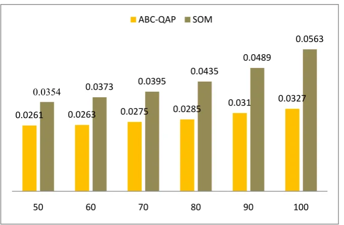
Fitness value,which calculates the coefficient
error ofpreserving of the approximately inherent structure of the data by dimension reduction, is 0.0327 and 0.0563 for QAP-ABC and SOM, respectively (Fig. 9). It can be clearly observed that the QAP-ABC has been better than SOM and
other used methods and 41% improvement in the fitness values over SOM.
In ABC, The onlooker ants select scout bees based on elite selection. The elite selection preserves the best solutions without any change in next step. The transforming of the best solutions to next step and the ignorance of the worst solutions cause to search increase
for bees in the high fitness region of the state
space, increases thus improving exploitation. Moreover, number of soldier bees is determined
based on the fitness of scout bees. Thus the best
scout bees have more soldier bees for search. It result concentrate to better promising region of search space (exploitation) and decrease the computational time and increase the convergence speed.This is because the QAP-ABC increasesthe exploitation from information of meet points by using of positive feedback. It should also be noted that QAP-ABC has higher computational time compared with SOM.
VI. CONCLUSION
In this work we suggested a new approach
based on Artificial Bee Colony and Quadric
data set with same circumstances. The results were compared and it showed that QAP-ABC has high performance with compared others.
Table 3. The data visualization precise of various approaches Dataset
size
QAP-ABC SOM Sammon's Map MDS
Fitness RunningTime Fitness RunningTime Fitness RunningTime Fitness RunningTime
50 0.0261 3215 0.0354 732 0.0262 12040 0.0264 11510
60 0.0263 4587 0.0373 762 0.0265 12350 -
-70 0.0275 6051 0.0395 775 - - -
-80 0.0285 7562 0.0435 782 - - -
-90 0.031 8541 0.489 793 - - -
-100 0.0327 10578 0.0563 1015 - - -
-0.0261 0.0263 0.0275 0.0285 0.031
0.0327
0.0354 0.0373 0.0395
0.0435 0.0489
0.0563
50 60 70 80 90 100
ABC-QAP SOM
REFERENCES
[1] L. Xu, Y. Xu, T. W. S. Chow, “PolSOM: A new method for multidimensional data visualization”, Pattern Recognition, Volume 43, Issue 4, pp. 1668–1675, 2010.
[2] Y. Xu, L. Xu, T. W. S. Chow, “PPoSOM: A new variant of PolSOM by using probabilistic assignment for multidimensional data visualization”, Neurocomputing, Volume 74, Issue 11, pp. 2018–2027, 2011.
[3] F. S. Tsai, “Dimensionality reduction techniques for blog visualization”, Expert Systems with Applications, Volume 38, Issue, pp. 2766–2773, 2011.
[4] R. Abbiw-Jackson, B. Golden, S. Raghavan, and E. Wasil, “A divide-and-conquer local search heuristic for data visualization”, Computers and operations research, Volume 33, Issue 11, pp. 3070–3087, 2006.
[5] M. H. Ghaseminezhad, A. Karami, “A novel self-organizing map (SOM) neural network for discrete groups of data clustering”, Applied Soft Computing, Volume 11, Issue 4, pp. 3771–3778, 2011.
[6] P. Klement, V. Snášel, “Using SOM in the performance monitoring of the emergency call-taking system”, Simulation Modelling Practice and Theory, Volume 19, Issue 1, pp. 98–109, 2011.
[7] J. W. Sammon, “A nonlinear mapping for data structure analysis”, IEEE Transactions on computers, Volume 18, Issue 5, pp. 401–409, 1969.
[8] J. Sun, C. Fyfe, M. Crowe, “Extending Sammon mapping with Bregman divergences”, Information Sciences, Volume 187, pp. 72–92, 2012.
[9] G. Gan, C. Ma, J. Wu, Data Clustering: Theory, Algorithms, and Applications, Society for Industrial and Applied Mathematics, 2007.
[10] P. A. De Mazière, M. M. Van Hulle, “A clustering study of a 7000 EU document inventory using MDS and SOM”, Expert Systems with Applications, Volume 38, Issue 7, pp. 8835–8849, 2011.
[11] M. Ghanbari, “Visualization Overview”, Thirty-Ninth Southeastern Symposium on System Theory, pp. 115–119, 2007.
[12] S.-H. Bae, J. Qiu, G. Fox, “Adaptive interpolation of multidimensional scaling”, Procedia Computer Science, Volume 9, pp. 393–402, 2012.
[13] A. M. Lopes, J. A. Tenreiro Machado, C. M. A. Pinto, and A. M. S. F. Galhano, “Fractional dynamics and MDS visualization of earthquake phenomena”, Computers & Mathematics with Applications, Volume 66, Issue 5, pp. 647–658, 2013.
[14] T. Kohonen, “The self-organizing map”, Neurocomputing, Volume 21, Number 1-3, pp. 1–6, 1998.
[15] H. T. Jadhav, R. Roy, “Gbest guided artificial bee colony algorithm for environmental/economic dispatch considering wind power”, Expert Systems with Applications, Volume 40, Issue 16, pp. 6385–6399, 2013.
[16] A. P. Engelbrecht, Computational Intelligence: An Introduction, Wiley, 2007.
[17] C. B. Kalayci, S. M. Gupta, “Artificial bee colony algorithm for solving sequence-dependent disassembly line
balancing problem”, Expert Systems with Applications, Volume 40, Issue 18, pp. 7231–7241, 2013.
[18] H.-C. Tsai, “Integrating the artificial bee colony and bees algorithm to face constrained optimization problems”, Information Sciences, Volume 258, pp. 80–93, 2013.
[19] J.-Y. Park, S.-Y. Han, “Application of artificial bee colony algorithm to topology optimization for dynamic stiffness problems”, Computers & Mathematics with Applications, Volume 66, Issue 10,, pp. 1879–1891, 2013.
[20] M. Rani, H. Garg, S. P. Sharma, “Cost minimization of butter-oil processing plant using artificial bee colony technique”, Mathematics and Computers in Simulation, Volume 97, pp. 94–107, 2014.
[21] V. Golmah, J. Parvizian, “Visualization and the understanding of multidimensional data using Genetic Algorithms: Case study of load patterns of electricity customers”, International Journal of Database Theory & Application, Volume 3, Issue 4, pp. 41–56, 2010.
[22] J. Vesanto, J. Himberg, E. Alhoniemi, J. Parhankangas, S. Team, and L. Oy, “Som toolbox for matlab 5”, Technical Report A57, Helsinki University of Technology,Neural Networks Research Centre,2000.