Iterative Weighted Non-smooth Non-negative Matrix Factorization for Face Recognition

Please cite this article as: B. Sabzalian, V. Abolghasemi, Iterative Weighted Non-smooth Non-negative Matrix Factorization for Face Recognition , International Journal of Engineering (IJE), IJE TRANSACTIONS A: Basics Vol. 31, No. 10, (October 2018) 1698-1707

International Journal of Engineering

Faculty of Electrical Engineering and Robotics, Shahrood University of Technology, Shahrood, Iran

P A P E R I N F O

Paper history:

Received 04 March 2018

Received in revised form 16 August 2018 Accepted 18 August 2018

Keywords:

Non-negative Matrix Factorization Face Recognition

Pattern Analysis Features Extraction Sparse Representation

A B S T R A C T

Non-negative Matrix Factorization (NMF) is a part-based image representation method. It comes from the intuitive idea that entire face image can be constructed by combining several parts. In this paper, we propose a framework for face recognition by finding localized, part-based representations, denoted “Iterative weighted non-smooth non-negative matrix factorization” (IWNS-NMF). A new cost function is proposed in order to incorporate sparsity which is controlled by a specific parameter and weights of feature coefficients. This method extracts highly localized patterns, which generally improves the capability of face recognition. After extracting patterns by IWNS-NMF, we use principle component analysis to reduce dimension for classification by linear SVM. The Recognition rates on ORL, YALE and JAFFE datasets were 97.5, 93.33 and 87.8%, respectively. Comparisons to the related methods in the literature indicate that the proposed IWNS-NMF method achieves higher face recognition performance than NMF, NS-NMF, Local NMF and SNMF.

doi: 10.5829/ije.2018.31.10a.12

1. INTRODUCTION1

Face recognition has been considered as one of the most challenging problems in computer vision and image processing communities since two decades ago. A well-established and widely used method in face recognition is Eigen face [1] which is based on principle component analysis (PCA). It is performed directly on the entire patterns in order to extract the global feature vectors which are later utilized for classification task. As a result, the classification is achieved by a set of previously found global projectors from an existing training pattern set. The objective of this process is to achieve a mostly adequate subspace for face representation and recognition. However, there are many applications where localized features provide benefits for object recognition, such as stability to local deformations, partial occlusion, and lighting variations. Traditionally, PCA and LDA (Linear Discriminant Analysis) [2] have been the standard approaches to reduce the high-dimensional original pattern vector space into low-dimensional feature vector space [3]. A decade ago, an approach for obtaining a part-based linear representation of the facial

*Corresponding Author Email: [email protected] (V. Abolghasemi)

image has been proposed. This technique is known as Non-negative Matrix Factorization (NMF), firstly introduced by Lee and Seung [4]. NMF is an unsupervised method, solving real world problems with non-negative data. NMF has been widely used for many tasks such as data mining [5, 6], pattern recognition [7, 8], and computer vision [9, 10]. In what follows, we briefly review some of the important NMF techniques. A new multiplicative update algorithm was proposed by Li, et al. [11] that minimizes the Euclidean distance between approximate and true values in original NMF cost function. It is proved that this algorithm converges faster than existing ones to a stationary point. In another work, a novel NMF method was proposed under noisy separability conditions. The proposed method reported in literature [12] is called ellipsoid-volume minimization based on NMF. It seeks for a minimum-volume ellipsoid centered at the origin and encloses the data columns x1,

…, xn and their mirrors -x1, …, -xn. Then, under

separability condition, the minimum-volume enclosing ellipsoid touches the data cloud at ±W(:,r) for r = 1,...,R. Zhang et al. proposed a correntropy supervised NMF (CSNMF) to mitigate the existing deficiencies [13]. The

Iterative Weighted Non-smooth Non-negative Matrix Factorization for Face

Recognition

approach is to maximize correntropy between the data matrix and reconstruction space. Conversely, CSNMF minimizes correntropy between two coefficients that have the same class labels. Non-negative matrix factorization (NMF) is applied over data distribution for linear discriminant analysis which achieves good results [14]. A graph regularize non-negative matrix factorization (GNMF) was proposed in literature [15], which has been later improved by Wang et al. [16]. They proposed graph regularized matrix decomposition with sparse coding (GRNMF SC) which extracts the basis vectors through the data space. An algorithm was proposed in literature [17] that improves the ability of new representation using class labels. Use of these labels, data samples can be divided into within-class and between-class features. Extreme Learning Machine (ELM) is a fast algorithm for Single-hidden Layer Feed-forward Neural (SLFN) networks training that requires low human supervision [18]. Iosifidis et al. [19] propose a novel approximate kernel ELM (noted as AKELM hereafter) formulation. They demonstrated that the proposed approach performs extremely fast, comparing to the kernel ELM approach. At the same time, it achieves comparable performance with that of kernel ELM. A novel algorithm, called Optimal Expression-specific Parts Accumulation (OEPA), was also proposed by Ali et al. [20] which accumulates the subset of facial parts. It divides the face images into four facial parts (Left eye, Right eye, Mouth, Nose). It then calculates which part is responsible for describing a specific expression. Li et al. [21] developed a novel NMF algorithm with fast convergence rate and high performance. This method takes advantages of choosing the step-length which is constrained to be greater than that of conventional NMF. In another facial application, Wang [22] proposed the block diagonal non-negative matrix factorization (BDNMF) for color face representation and recognition. The approach uses block diagonal matrix with the aim of interpreting color information of various channels. In another work, the authors proposed a hybrid technique by combining Gabor Wavelet and Non-negative Matrix Factorization [23]. In this method, each image was independently processed and then convolved with Gabor kernel. Then, after feature extraction, the matrix dimensionality was reduced using NMF. Chen et al. [24] proposed a supervised kernel NMF for face recognition. The SKNMF compresses the within-class features and takes apart the between-class features. Liu and Wechsler [25] proposed a method using Fisher Linear Discriminant Analysis (FLDA), called Fisher Non-negative Matrix Factorization (FNMF). This method adds fisher constraint to the traditional NMF to maximize between class features and minimize within class ones. In this paper, we proposed a new iterative approach to solve face recognition problem with the sparsity constraint on both factorized matrices. The proposed method is an iterative

weighted smoothing function in order to preserve strong features and to suppress the weak features. In fact, the main goal of IWNS-NMF is to find sparse structures that strengthen features according to their coefficient in the basis functions, which facilitates the subsequent classification process.

The rest of the paper is organized as follows. In Section 2, we mathematically represent the original NMF framework and its variants. In Section 3, the proposed model in this paper is presented. In Section 4 the experimental results of applying different methods are given and compared. Finally, the conclusion is drawn in Section 5.

2. NON-NEGATIVE MATRIX FACTORIZATION AND ITS VARIANTS

2. 1. Non-negative Matrix Factorization (NMF)

Non-negative Matrix Factorization is composed of a group of multivariate rules based on linear algebra where a matrix V is factorized into two matrices W and H. Let matrix V be the product of the matrices W and H [4],

𝑉 ≈ 𝑊 × 𝐻 (1)

where 𝑉 ∈ ℛ𝑝×𝑛 _{is the input matrix with p rows and n}

columns, 𝑊 ∈ ℛ𝑝×𝑞and 𝐻 ∈ ℛ𝑞×𝑛are called the basis and encoding vectors, respectively. To find an approximate factorization𝑉 ≈ 𝑊𝐻 we first need to define a cost function that quantifies the quality of the approximation. This can be achieved using some measure of distance between two non-negative matrices A and B. One useful measure is simply the square of the Euclidean distance between A and B.

‖𝐴 − 𝐵‖2_{= ∑ (𝐴}

𝑖𝑗− 𝐵𝑖𝑗)2

𝑖𝑗 (2)

This is lower bounded by zero, and clearly vanishes if and only if A = B. Another useful measure is

𝐷(𝐴 ∥ 𝐵) = ∑ (𝐴𝑖𝑗log

𝐴𝑖𝑗

𝐵𝑖𝑗− 𝐴𝑖𝑗+ 𝐵𝑖𝑗)

𝑖𝑗 (3)

Similar to Euclidean distance, this measure is also lower bounded by zero, and vanishes if and only if A = B. However, it cannot be called a “distance”, since it is not symmetric in A and B. Hence, the term “divergence” of A from B is commonly used. It reduces to the Kullback-Leibler divergence, or relative entropy, when ∑ 𝐴𝑖𝑗 𝑖𝑗=

∑ 𝐵𝑖𝑗 = 1 , so that A and B can be regarded as

normalized probability distributions.

As mentioned before all three matrices have non-negative elements, and the columns of W are commonly normalized. Using Poisson likelihood the following objective function can be designed:

𝐷(𝑉, 𝑊𝐻) = ∑ ∑ (𝑉𝑖𝑗𝑙𝑛

𝑉𝑖𝑗

(𝑊𝐻)𝑖𝑗− 𝑉𝑖𝑗+ (𝑊𝐻)𝑖𝑗)

𝑛 𝑗=1 𝑝

where it can be converted to (5) after some simplifications:

𝐷(𝑉, 𝑊𝐻) = ∑𝑝𝑖=1∑𝑛𝑗=1(∑𝑞𝑘=1𝑊𝑖𝑘− 𝑉𝑖𝑗𝑙𝑛 ∑𝑞𝑘=1𝑊𝑖𝑘𝐻𝐾𝑗) (5)

In order to solve (5), one simple method is to alternatively updating W and H by considering their derivatives. If we take the derivative with respect to H the following equation can be obtained:

𝜕

𝜕𝐻𝑎𝑏𝐷(𝑉, 𝑊𝐻) = ∑ 𝑊𝑖𝑎

𝑝

𝑖=1 − ∑

𝑉𝑖𝑏𝑊𝑖𝑎

∑𝑞𝑘=1𝑊𝑖𝑘𝐻𝑘𝑏

𝑝

𝑖=1 (6)

Then, using the gradient descent algorithm, H can be obtained:

𝐻𝑎𝑏= 𝐻𝑎𝑏− 𝜂𝑎𝑏_𝜕𝐻𝜕

𝑎𝑏𝐷(𝑉, 𝑊𝐻) (7)

𝐻𝑎𝑏= 𝐻𝑎𝑏+ 𝜂𝑎𝑏[∑ _∑ 𝑉𝑖𝑏_𝑊𝑊𝑖𝑎

𝑖𝑘𝐻𝑘𝑏

𝑞

𝑘=1 − ∑ 𝑊𝑖𝑎

𝑝 𝑖=1 𝑝

𝑖=1 ] (8)

where ɳab is the step-size and can be defined such as:

𝜂𝑎𝑏=_∑𝐻𝑎𝑏_𝑊

𝑖𝑎 𝑝 𝑖=1

(9)

Another form of update equation is using the multiplicative rules [4]:

𝐻𝑎𝑏= 𝐻𝑎𝑏

∑𝑝𝑖=1(𝑊𝑖𝑎𝑉𝑖𝑏)

∑𝑞𝑘=1𝑊𝑖𝑘𝐻𝑘𝑏

⁄ ∑𝑝𝑖=1𝑊𝑖𝑎

(10)

The same steps can be written for W. By computing the derivative of Equation (10) with respect to W

𝜕

𝜕𝑊𝑐𝑑𝐷(𝑉, 𝑊𝐻) = ∑ 𝐻𝑑𝑗− ∑

𝑉𝑐𝑗𝐻𝑑𝑗

∑𝑞𝑘=1𝑊𝑐𝑘𝐻𝑘𝑗

𝑛 𝑗=1 𝑛

𝑗=1 (11)

The gradient method:

𝑊𝑐𝑑= 𝑊𝑐𝑑− 𝑉𝑐𝑑_𝜕𝑊𝜕

𝑐𝑑𝐷(𝑉, 𝑊𝐻) (12)

𝑊𝑐𝑑= 𝑊𝑐𝑑+ 𝑉𝑐𝑑[∑ 𝑉𝑐𝑗

𝐻𝑑𝑗

∑𝑞𝑘=1𝑊𝑐𝑘𝐻𝑘𝑗

𝑛

𝑗=1 − ∑𝑛𝑗=1𝐻𝑑𝑗] (13)

The step size:

𝑉𝑐𝑑=_∑𝑊𝑐𝑑_𝐻

𝑑𝑗 𝑛

𝑗=1 (14)

Gives:

𝑊𝑐𝑑= 𝑊𝑐𝑑

∑𝑛𝑗=1(𝐻𝑑𝑗𝑉𝑐𝑗)

∑𝑞𝑘=1𝑊𝑐𝑘𝐻𝑘𝑗

⁄

∑𝑛𝑗=1𝐻𝑑𝑗

(15)

Formally, the detailed algorithm can be represented as follows:

Repeat until convergence: For a = 1...q do begin For b = 1...n do

𝐻𝑎𝑏= 𝐻𝑎𝑏

∑𝑝𝑖=1(𝑊𝑖𝑎𝑉𝑖𝑏)

∑𝑞𝑘=1𝑊𝑖𝑘𝐻𝑘𝑏

⁄

∑𝑝_𝑖=1𝑊_𝑖𝑎

(16)

For c=1...p do begin

𝑊𝑐𝑎= 𝑊𝑐𝑎

∑ (𝐻𝑎𝑗𝑉𝑐𝑗)_∑

𝑊𝑐𝑘𝐻𝑘𝑗 𝑞 𝑘=1

⁄

𝑛 𝑗=1

∑𝑛𝑗=1𝐻𝑎𝑗

(17)

𝑊𝑐𝑎=_∑𝑊𝑐𝑎_𝑊

𝑗𝑎 𝑛

𝑗=1 (18)

End End

2. 2. Local Non-negative Matrix Factorization

(LNMF) The Local Non-negative Matrix Factorization

(LNMF) algorithm was proposed by Feng et al. [26]. This algorithm aimed at learning localized, part-based features in W for a factorization V=WH. It forces the sparseness constraints on coefficient matrix H and locally constraints on feature basis matrix W. Considering the problem given in Equation (1), we set aij = WtW and B =

bij = HHt, where 𝐴, 𝐵 ∈ ℛ𝑞×𝑞. The following steps define

the existing constraints in LNMF algorithm:

1. Maximization of sparsity in H.H should have its most samples nearly zero and contain few non-zeros. This corresponds to minimization of basis elements. This is achieved by minimization of all aij.

2. Maximization of expressiveness in W. This constraint is directly connected to the previous step. In other words, it is designed to incorporate maximum sparsity in H. Mathematically, ∑𝑞_𝑖=1b_𝑖𝑖 should be maximized.

3. Maximum orthogonality of W. This constraint is considered in order to make the basis as orthogonal as possible and consequently to minimize the redundancy. This is achieved by minimizing ∑_{∀𝑖,𝑗,𝑖≠𝑗}𝑎_𝑖𝑗 . Combination of this constraint with stage 1 leads to an expression to minimize ∑∀𝑖,𝑗𝑎𝑖𝑗.Such incorporation of

the above constraints can be compactly written as the following divergence functions for LNMF:

𝐷(𝑉, 𝑊𝐻) = ∑ ∑ (𝑉𝑖𝑗𝑙𝑛_(𝑊𝐻)𝑉𝑖𝑗

𝑖𝑗− 𝑉𝑖𝑗+

𝑛 𝑗=1 𝑝 𝑖=1

(𝑊𝐻)𝑖𝑗) + 𝛼 ∑𝑖,𝑗=1𝑞 (𝑊𝑇𝑊)𝑖𝑗− 𝛽 ∑𝑞𝑖,𝑗=1(𝐻𝐻𝑇)𝑖𝑗

(19)

where 𝛼, 𝛽 > 0 are constant scalars. These values can control the effect of additional constraints defined above. Using the following update rules, the LNMF algorithm is minimized.

Repeat until convergence: For a =1...q do begin For b = 1...n do

𝐻𝑎𝑏= √𝐻𝑎𝑏∑ (𝑊𝑖𝑎𝑉𝑖𝑏)/ ∑𝑞𝑘=1𝑊𝑖𝑘𝐻𝑘𝑏

𝑝

𝑖=1 (20)

For c = 1...p

Update basis matrix Wusing Equations (17) and (18) End

2. 3. Sparse Non-negative Matrix Factorization

the method presented in literature [28]. Hoyer [28] used Kullback-Leibler (DKL) divergence term instead of Euclidean least-square term as used in the original NMF [4]. Thus, the objective function of SNMF [27] is defined as follows:

𝐷(𝑉, 𝑊𝐻) = ∑ ∑ (𝑉𝑖𝑗𝑙𝑛

𝑉𝑖𝑗

(𝑊𝐻)𝑖𝑗− 𝑉𝑖𝑗+

𝑛 𝑗=1 𝑝 𝑖=1

(𝑊𝐻)𝑖𝑗) + 𝛼 ∑ 𝐻𝑖𝑗 𝑖𝑗

(21)

where 𝛼 ≥ 0 is a constant, 𝑉, 𝑊, 𝐻 ≥ 0. Using the following updates rules, the SNMF algorithm is minimized:

𝐻𝑎𝑏= 𝐻𝑎𝑏

∑𝑝𝑖=1(𝑊𝑖𝑎𝑉𝑖𝑏)

∑𝑞𝑘=1𝑊𝑖𝑘𝐻𝑘𝑏

⁄

1+𝛼

(22)

The Equations (17) and (18) were used to update basis matrix W.

2. 4. Subclass Discriminant Non-negative Matrix

Factorization (SDNMF) Nikitidis et al. [14] extend

the NMF algorithm by modifying the decomposition using appropriate discriminant penalties. This method provides discriminant projections leading to both robustness against illumination changes and expression variations. It also enhances class separability in the reduced dimensional space.

In this method, Subclass based discriminant constraints are incorporated in the NMF cost function leading to a specialized NMF-based method. Novel multiplicative update rules are used for optimizing SDNMF. The corresponding cost function for the SDNMF problem is represented as follows:

𝐷𝑆𝐷𝑁𝑀𝐹 (𝑉||𝑊𝐻) ≜ 𝐷𝑁𝑀𝐹(𝑉||𝑊𝐻) + 𝛼

2𝑡𝑟[∑ ]𝑤 −

𝛽

2𝑡𝑟[∑ ]𝑤

(23)

where α and β are positive constants, while 1/2 is used to simplify subsequent derivations. Where tr[∑ ]𝑤 is the

matrix trace operator. The update rule for the weight coefficients ℎ𝑘,𝑙 which for the t-th iteration is defined as

ℎ_𝑘,𝑙(𝑡)=

𝐴+√𝐴2_{+4(𝛼−[𝛼+} 𝛽

𝑁(𝑟)(𝜃)(𝐶−𝐶𝑟)]_{𝑁(𝑟)(𝜃)}1 )ℎ𝑘,𝑙(𝑡−1)∑ 𝑤𝑖,𝑘(𝑡−1) 𝑣𝑖,𝑙

∑ 𝑤𝑖,𝑛𝑛 (𝑡−1)ℎ𝑛,𝑙(𝑡−1)

𝑖

2(𝛼−[𝛼+ 𝛽

𝑁(𝑟)(𝜃)(𝐶−𝐶𝑟)]

1

𝑁(𝑟)(𝜃))

(24)

here ℎ𝑘,𝑙 can be also considered as the k-th feature

element, in the projection subspace, of the l-th image belonging to the y-th cluster of the r-th facial class, 𝐶𝑟 is

the number of subclasses composing the r-th class , C is the total number of formed subclasses in the database and parameter A is defined as:

𝐴 = (𝛼 +_𝑁𝛽

(𝑟)(𝜃)(𝐶 − 𝐶𝑟)

1

𝑁(𝑟)(𝜃)∑ ℎ𝑘,𝜆

(𝑡−1)

−

𝜆,𝜆≠1 𝛽

𝑁(𝑟)(𝜃)∑ ∑ 𝜇

(𝑚)(𝑔)_{− 1} 𝑐𝑚

𝑔=1 𝑛

𝑚,𝑚≠𝑟

(25)

For more info and a proof that the objective function is guaranteed to have a non-increasing behavior can be found in [14].

2. 5. Non-Smooth Non-Negative Matrix

Factorization (nsNMF) Pascual-Montano et al. [8]

proposed a method for optimizing a cost function which is designed for expressing sparsity in the form of non-smoothness controlled by a parameter. The model proposed in [8] is defined as:

𝑉 ≈ 𝑊𝑆𝐻 (26)

where V, W, and H are input data, basis, and coefficient matrices, respectively. The positive symmetric matrix

𝑆 ∈ 𝑅𝑞×𝑞 _{is a smoothing matrix defined as:}

𝑆 = (1 − 𝜃)𝐼 +𝜃_𝑞11𝑇 ₍₂₇₎

I is the identity matrix, 1is a vector of all ones, and variable θ meets 0 <θ< 1. More details about the algorithm and pseudo-code can be read from [8].

3. PROPOSED ITERATIVE WEIGHTED NON-SMOOTH NMF (IWNS-NMF)

One of the main drawbacks of nsNMF is leaving weak features that do not contribute significantly in the classification process. In fact, if one can gradually assess the features strength and remove those that are insignificant the resultant classification rate will be increased. To do this, here we propose a modification to nsNMF method for facial recognition called Iterative Weighted nsNMF (IWNS-NMF).The schema of the proposed method is shown in Figure 1.The objective is to apply sparseness to both the basis and encoding vectors which is defined by Equation (27). The proposed algorithm is:

Repeat until convergence: For a = 1...q do begin For b = 1...n do

𝐻𝑎𝑏= 𝐻𝑎𝑏

∑𝑝𝑖=1((𝑊𝑖𝑎𝑆)𝑉𝑖𝑏)

∑𝑞𝑘=1(𝑊𝑖𝑘𝑆)𝐻𝑘𝑏

⁄ ∑𝑝𝑖=1(𝑊𝑖𝑎𝑆)

(28)

For c=1...p do begin

𝑊𝑐𝑎= 𝑊𝑐𝑎

∑ ((𝐻𝑎𝑗𝑆)𝑉𝑐𝑗)

∑𝑞𝑘=1(𝑊𝑐𝑘𝑆)𝐻𝑘𝑗

⁄

𝑛 𝑗=1

∑𝑛𝑗=1(𝑆𝐻𝑎𝑗)

(29)

𝑊𝑐𝑎=_∑𝑊𝑐𝑎_𝑊

𝑗𝑎 𝑛

𝑗=1 (30)

End End

𝑆 = (1 − 𝐼𝑡𝑒𝑟_𝜃)𝐼 +𝐼𝑡𝑒𝑟_𝜃_𝑞 11𝑇 ₍₃₁₎

𝐼𝑡𝑒𝑟_𝜃 is the smooth parameter that is updated in each iteration that defines as:

𝐼𝑡𝑒𝑟_{𝜃𝑖= 𝑖 (𝜃 𝑀𝑎𝑥}

𝑖𝑡𝑒𝑟

⁄ )

𝑖 = 0,1, … , 𝑀𝑎𝑥_𝑖𝑡𝑒𝑟

(32)

I,1 and θ are defined above. 𝑖 and 𝑀𝑎𝑥_𝑖𝑡𝑒𝑟, are iteration index and the maximum number of iterations respectively. As mentioned before,𝐼𝑡𝑒𝑟_𝜃𝑖 increments

within [0 , 𝜃] at various iterations, leading to changes in the elements of smooth matrix S. It is important to note that we propose weighted smoothing function using the iterative smooth matrix that keeps and strengthens important features and weakens or removes insignificant features, iteratively and gradually. In contrast, the smooth matrix S in [8] has constant elements depending on a fix θ which cannot adaptively control the smoothness. Therefore, it is not possible to control the feature coefficients and to check which feature is more important to be sparse. This has been resolved by the proposed method in this paper. In other words, the proposed S matrix has dynamic elements depending on θ and iteration number, which calculates weights of H and then multiplied by S. This procedure causes strong features to become stronger and reversely weak features to become weaker.

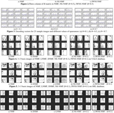
As shown in our experimental results, the proposed method outperforms NS-NMF and provides improved sparsity conditions. Figure 2 shows three columns of H matrix in NMF, NS-NMF (θ=0.5), and IWNS-NMF(θ=0.5) algorithms. It is obvious that IWNS-NMF keeps the strong features with higher coefficient and remove or weaken the undesirable features (notice the low-amplitude coefficients in both graphs in Figure 2).

4. EXPERIMENTS

The experiments for face recognition application were conducted for two well-known databases, the ORL 48 × 48 database and YALE 32 × 32 databases. The ORL [29] is composed of 400 images, 10 different images per person for 40 persons. For some individuals, the images were acquired at different times. The facial expressions in these images are different, e.g. open or closed eyes and smiling or non-smiling. Other facial details such as glasses or no glasses also exist.

Figure 1. IWNS-NMF face recognition algorithm diagram

YALE [2] database is more challenging than ORL. It has 165 gray-scale images of 15 individuals. The images introduce various lighting condition such as left-light, center-light, and right-light. It also represents facial expressions, e.g. normal, happy, sad, sleepy, and surprised. Similar to ORL it has facial details as glasses or no glasses. The Japanese Female Facial Expressions (JAFFE) dataset [30] consists of 213 grayscale images presenting seven facial expressions (happiness, sadness, fear, anger, surprise, disgust, and neutrality (that were posed by 10 Japanese female models. Each image size is of 256 × 256 pixels, and each model has 2–4 samples for each expression. Each cropped facial image in the datasets was isotopically scaled to the fixed size of 32 × 32 pixels. These algorithms are utilized here for comparing with the proposed method: NMF [4], LNMF [26], SNMF [27], and NS-NMF [8]. In these simulations, a metric called “sparseness metric” (SP) [31] are used to evaluate the sparsity of basis matrix as well as coefficients matrix. SP, which is defined as a combination of L1 norm and the L2 norm, is written as follows

𝑆𝑃(𝐻) =

√𝑁−(∑|ℎ𝑖|

√∑ ℎ𝑖2

⁄ )

√𝑁−1

(33)

where h𝑖 is i-th column of matrix H. If all samples of h𝑖

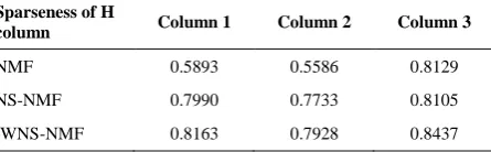
are the same, SP(H) would be zero; if h𝑖 contains merely one nonzero sample, SP(H) would become one. In addition, N is the number of elements in a vector. Table-1 shows the sparseness of these columns. In this table, we see that sparseness value of IWNS-NMF is higher than NS-NMF and NMF. NMF family methods should lead to decomposition matrix V into the matrix W and H. In each iteration, W and H are updated until convergence. After feature extraction by IWNS-NMF, they are projected to higher features variance axes to calculate eigen values by PCA and to reduce dimension. These features are then ready for classification, in which linear SVM kernel is used. The classification results are presented next.

IWNS-NMF was evaluated on the ORL facial database. Different sparseness parameters, i.e. 0.1, 0.3 and 0.7, were used with 60 features. The reason of giving this example is to make the effects of signals sparsity visible (while increasing θ).

TABLE 1. The sparseness of three column Of H matrix in

NMF, NS-NMF (Θ=0.5), IWNS-NMF (Θ=0.5)

Sparseness of H

column Column 1 Column 2 Column 3

NMF 0.5893 0.5586 0.8129

NS-NMF 0.7990 0.7733 0.8105

Figure 3 shows the results. These results show the effect of IWNS-NMF to achieve more localized features while increasing the sparseness parameter. Increasing the value of θ corresponds to sparse encoding vectors. Figures 4, 5 and 6 show the basis images of NMF, LNMF, SNMF,

NS-NMF (θ=0.1), IWNS-NMF (θ=0.1) on YALE, ORL, and JAFEE database. And Figures 7, 8 and 9 shows the five reconstruction effects by NMF, LNMF, SNMF, NS-NMF (θ=0.1), IWNS-NS-NMF (θ=0.1) on YALE, ORL and JAFEE databases respectively.

a) NMF b) NS-NMF c) IWNS-NMF

Figure 2.Three column of H matrix in NMF, NS-NMF (θ=0.5), IWNS-NMF (θ=0.5)

(a) θ = 0.1 (b) θ=0.3 (c) θ=0.7

Figure 3. Encoding vectors for 25 sample images and different values of sparseness: (a) θ=0:1, (b) θ= 0:3, (c) θ= 0:7.

a) NMF b) SNMF c) LNMF d) NS-NMF – (θ=0.1) e) IWNS-NMF – (θ=0.1)

Figure 4. 3×3 basis images of NMF, LNMF, SNMF, NS-NMF (θ=0.1), IWNS-NMF (θ=0.1) on YALE database.

a) NMF b) SNMF c) LNMF d) NS-NMF – (θ=0.1) e) IWNS-NMF – (θ=0.1)

Figure 5. 3×3 basis images of NMF, LNMF, SNMF, NS-NMF (θ=0.1), IWNS-NMF (θ=0.1) on ORL database.

a) NMF b) SNMF c) LNMF d) NS-NMF – (θ=0.1) e) IWNS-NMF – (θ=0.1)

a) original (32 × 32) b) NMF c) SNMF d) LNMF e) NS-NMF(θ=0.1) f) IWNS-NMF(θ=0.1)

Figure 7. Three reconstruction effects by NMF, LNMF, SNMF, NS-NMF (θ=0.1), IWNS-NMF (θ=0.1) on YALE database.

a) original (32 × 32) b) NMF c) SNMF d) LNMF e) NS-NMF(θ=0.1) f) IWNS-NMF (θ=0.1)

Figure 8. Three reconstruction effects by NMF, LNMF, SNMF, NS-NMF (θ=0.1), IWNS-NMF (θ=0.1) on ORL database.

a) original (32 × 32) b) NMF c) SNMF d) LNMF e) NS-NMF(θ=0.1) f) IWNS-NMF (θ=0.1)

Figure 9. Three reconstruction effects by NMF, LNMF, SNMF, NS-NMF (θ=0.1), IWNS-NMF (θ=0.1) on JAFFE database.

According to Sokolova and Lapalme [32] we compared recall and precision curves by following equations between IWNS-NMF and nsNMF.

𝑃𝑟𝑒𝑐𝑖𝑠𝑖𝑜𝑛 = ∑

𝑇𝑃𝑖 𝑇𝑃𝑖+𝐹𝑃𝑖 𝐿 𝑖=1

𝐿 (34)

𝑅𝑒𝑐𝑎𝑙𝑙 = ∑

𝑇𝑃𝑖 𝑇𝑃𝑖+𝐹𝑁𝑖 𝐿 𝑖=1

𝐿 (35)

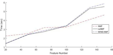
where TP is the number of true positives, FP is the number of false positives; FN is the number of true negatives, while L is the number of classes in dataset. In information retrieval, precision is a measure of result relevancy, while recall is a measure of how many truly relevant results are returned, so high precision relates to a low false positive rate, and high recall relates to a low false negative rate. High scores for both precision and recall indicate that the system is returning accurate results (high precision), as well as returning a majority of all positive results (high recall). In Figure 10, we compared methods in terms of computation time. The given values are convergence time after 100 iterations. According to this figure, the computation time of the proposed method is comparable to nsNMF and better than conventional

NMF. Figures 11 and 12 show the recall and precision curves in different feature number and theta parameter respectively. These curves show that our propose algorithm (IWNS-NMF) improve previous algorithm (NS-NMF) as well as possible.

Next, we list the best recognition rates of two face databases in Table 2. On ORL, YALE, and JAFEE, the samples of each individual are split into 6/4 for training/testing. The size of each subject is set to 50 for ORL, YALE, and JAFEE, and iteration number is 100 in IWNS-NMF.

After finding the best feature by PCA then we use linear SVM for classification. It shows that the IWNS-NMF is the best on both ORL, YALE and JAFEE datasets. For extra evaluation, the result of applying Convolutional Neural Network (CNN) has also been added to this table. CNN has a wide range of application especially in the field of image processing and pattern recognition [33]. A multilayer CNN (including input, convolutional, maxpooling, sigmoid, and softmax) was used for this purpose. As seen, although performance of CNN is comparable still the proposed method show higher recognition rate.

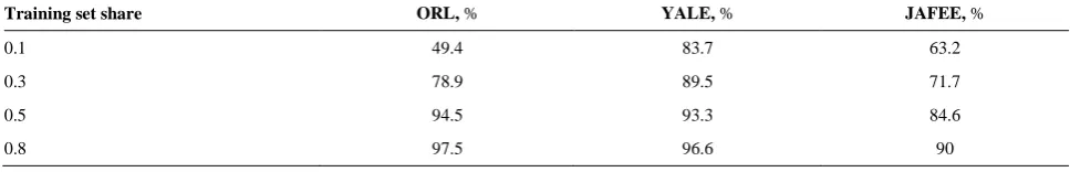
Finally, in Table 3 we demonstrate the recognition rate for different training set shares. For instance, “training set share =0.1” means 10% of total images are considered for training and the rest for test.In this experiment, the number of face images used for test and train is varied and the recognition rate was calculated in each case. As expected, when the size of training set is increases the performance is also improved. Moreover, the proposed algorithm is robust against changes in the dataset size and provides acceptable performance in average.

(a) (b)

Figure 11. Recall and precision applied to different feature

number and theta parameter in IWNS-NMF and NS-NMF (ORL Dataset).

(a) (b)

Figure 12. Recall and precision applied to different feature

number and theta parameter in IWNS-NMF and NS-NMF (YALE Dataset)

TABLE 2. Recognition rates on two face databases

Method ORL, % YALE, % JAFFE, %

IWNS-NMF + PCA 97.5 (θ=0.001) 93.33 (θ=0.2) 87.8 (θ=0.1)

NS-NMF + PCA 96.88 (θ=0.001) 90 (θ=0.2) 75.3 (θ=0.1)

NMF + PCA 95.00 88.33 66.7

LNMF + PCA 81.36 75 60.5

SNMF + PCA 93.33 90 69.1

CNN 93.21 89.82 68.5

SDNMF (c=2) [14] - 92.7 48.32

SDNMF (c=3) [14] - 90.1 49.26

AKELM [19] - - 60

TABLE 3. Recognition rates of the proposed method on two face databases for different variations in training set size

Training set share ORL, % YALE, % JAFEE, %

0.1 49.4 83.7 63.2

0.3 78.9 89.5 71.7

0.5 94.5 93.3 84.6

5. CONCLUSION

In this paper, we have presented a novel NMF method that attempts to augment the strong features and remove weak features during data decomposition process. This is achieved by taking part the weights of the coefficients, followed by PCA to decrease dimension of features. The experimental results on real datasets have demonstrated that the proposed IWNS-NMF algorithm is superior to traditional sparse NMF and its variants. We verified its performance for pattern classification with high dimension problem such as face recognition. As the future work, the following topics can be addressed; 1) this method works well for limited face conditions, thus, improving the method performance for recognizing face images in nonstandard conditions can be followed further; 2) its application for other data types, e.g. handwritten recognition, and 3) its performance for real-time application such as video face recognition could also be investigated in the future.

6. REFERENCES

1. Turk, M. and Pentland, A., “Eigenfaces for Recognition”,

Journal of Cognitive Neuroscience, Vol. 3, No. 1, (1991), 71–

86.

2. Belhumeur, P.N., Hespanha, J.P. and Kriegman, D.J., “Eigenfaces vs. Fisherfaces: Recognition Using Class Speciic Linear Projection”, IEEE Transactions on Pattern Analysis and

Machine Intelligence, Vol. 19, No. 7, (1997), 711–720.

3. Sadeghpour Haji, M., Mirbagheri, S.A., Javid, A.H., Khezri, M. and Najafpour, G.D., “A Wavelet Support Vector Machine Combination Model for Daily Suspended Sediment Forecasting”,

International Journal of Engineering - Transactions C:

Aspects, Vol. 27, No. 6, (2013), 855–864.

4. Lee, D.D. and Seung, H.S., “Learning the parts of objects by non-negative matrix factorization”, Nature, Vol. 401, No. 6755, (1999), 788–791.

5. Liu, C., Yang, H., Fan, J., He, L. and Wang Y.M., “Distributed non-negative matrix factorization”, United States patent US 8,356,086, (2013), https://patents.google.com/patent/US8356086B2/en.

6. Guan, N., Tao, D., Luo, Z.,. and Yuan, B., “NeNMF: An Optimal Gradient Method for Nonnegative Matrix Factorization”, IEEE

Transactions on Signal Processing, Vol. 60, No. 6, (2012),

2882–2898.

7. Li, S.Z., Hou, X.W., Zhang, H.J. and Cheng, Q.S., “Learning spatially localized, parts-based representation”, In Proceedings of the 2001 IEEE Computer Society Conference on Computer Vision and Pattern Recognition (CVPR 2001), IEEE, (2001). 8. Pascual-Montano, A., Carazo, J.M. , Kochi, K., Lehmann, D. and

Pascual-Marqui, R.D., “Nonsmooth Nonnegative Matrix Factorization (nsNMF)”, IEEE Transactions on Pattern

Analysis and Machine Intelligence, Vol. 28, No. 3, (2006), 403–

415.

9. Liu, H., Wu, Z., Cai, D. and Huang, T.S., “Constrained Nonnegative Matrix Factorization for Image Representation”,

IEEE Transactions on Pattern Analysis and Machine

Intelligence, Vol. 34, No. 7, (2012), 1299–1311.

10. Naiyang Guan, N., Dacheng Tao, D., Zhigang Luo, Z. and Bo

Yuan, B., “Online Nonnegative Matrix Factorization With Robust Stochastic Approximation”, IEEE Transactions on Neural

Networks and Learning Systems, Vol. 23, No. 7, (2012), 1087–

1099.

11. Li, L.X., Wu, L., Zhang, H.S. and Wu, F.X., “A Fast Algorithm for Nonnegative Matrix Factorization and Its Convergence”,

IEEE Transactions on Neural Networks and Learning Systems,

Vol. 25, No. 10, (2014), 1855–1863.

12. Mizutani, T., “Ellipsoidal Rounding for Nonnegative Matrix Factorization Under Noisy Separability”, The Journal of

Machine Learning Research , Vol. 15, No. 1, (2014), 1011–

1039.

13. Zhang, W., Guan, N., Tao, D., Mao, B., Huang, X. and Luo, Z., “Correntropy supervised non-negative matrix factorization”, In International Joint Conference on Neural Networks (IJCNN), IEEE, (2015), 1–8.

14. Nikitidis, S., Tefas, A., Nikolaidis, N. and Pitas, I., “Subclass discriminant Nonnegative Matrix Factorization for facial image analysis”, Pattern Recognition, Vol. 45, No. 12, (2012), 4080– 4091.

15. Nagipelli, N. and Eswar, K., “Graph Regularized Non-negative Matrix Factorization for Data Representation”, International

Journal of Computer Application, Vol. 03, No. 2, (2012), 171–

192.

16. Wang, B., Pang, M., Lin, C. and Fan, X., “Graph regularized non-negative matrix factorization with sparse coding”, In IEEE China Summit and International Conference on Signal and Information Processing, IEEE, (2013), 476–480.

17. Wang, J.J.Y. and Gao, X., “Max–min distance nonnegative matrix factorization”, Neural Networks, Vol. 61, (2015), 75–84. 18. Huang, G.B., Zhu, Q.Y. and Siew, C.K. “Extreme learning

machine: a new learning scheme of feedforward neural networks”, In IEEE International Joint Conference on Neural Networks, IEEE, (2004), 985–990.

19. Iosifidis, A., Tefas, A. and Pitas, I., “Approximate kernel extreme learning machine for large scale data classification”,

Neurocomputing, Vol. 219, , (2017), 210–220.

20. Ali, H.B., Powers, D.M.W., Jia, X. and Zhang, Y., “Extended Non-negative Matrix Factorization for Face and Facial Expression Recognition”, International Journal of Machine

Learning and Computing, Vol. 05, No. 2, (2015), 142–147.

21. Li, Y., Chen, W., Pan, B., Zhao, Y. and Chen, B., “An Efficient Non-negative Matrix Factorization with Its Application to Face Recognition”, In Chinese Conference on Biometric Recognition, Springer, (2015), 112–119.

22. Wang, C. and Bai, X., “Color Face Recognition Based on Revised NMF Algorithm”, In Second International Conference on Future Information Technology and Management Engineering, IEEE, (2009), 455–458.

23. Purnomo, F., Suhartono, D., Shodiq, M., Susanto, A., Raharja, S. and Kurniawan, R.W., “Face recognition using Gabor Wavelet and Non-negative Matrix Factorization”, In SAI Intelligent Systems Conference (IntelliSys), IEEE, (2015), 788–792. 24. Chen, W., Zhao, Y., Pan, B. and Xu, C., “Nonlinear Nonnegative

Matrix Factorization Based on Discriminant Analysis with Application to Face Recognition”, In 11th International Conference on Computational Intelligence and Security (CIS), IEEE, (2015), 191–194.

25. Liu, C. and Harry, W., “Robust Coding Schemes for Indexing and Retrieval from Large Face Databases”, IEEE Transactions on

Image Processing, Vol. 9, No. 1, (2000), 132–137.

27. Liu, W., Zheng, N. and Lu, X., “Non-negative matrix factorization for visual coding”, In IEEE International Conference on Acoustics, Speech, and Signal Processing Proceedings, (ICASSP ’03), IEEE, (2003).

28. Hoyer, P.O., “Non-negative sparse coding”, In Proceedings of the 12th IEEE Workshop on Neural Networks for Signal Processing, IEEE, (2002), 557–565.

29. Samaria, F.S. and Harter, A.C., “Parameterisation of a stochastic model for human face identification”, In Proceedings of 1994 IEEE Workshop on Applications of Computer Vision, IEEE, (1994), 138–142.

30. Dailey, M.N., Joyce, C., Lyons, M.J., Kamachi, M., Ishi, H., Gyoba, J. and Cottrell, G.W., “Evidence and a Computational Explanation of Cultural Differences in Facial Expression

Recognition”, Emotion, Vol. 10, No. 6, (2010), 874–893. 31. Chen, Y., Zhang, J., Cai, D., Liu, W. and He, X., “Nonnegative

Local Coordinate Factorization for Image Representation”, IEEE

Transactions on Image Processing, Vol. 22, No. 3, (2013), 969–

979.

32. Sokolova, M. and Lapalme, G., “A systematic analysis of performance measures for classification tasks”, Information

Processing & Management, Vol. 45, No. 4, (2009), 427–437.

33. Khatami, A., Babaie, M., Tizhoosh, H.R., Nazari, A., and Khosravi, A., “A Radon-based Convolutional Neural Network for Medical Image Retrieval”, International Journal of

Engineering-Transactions C: Aspects, Vol. 31, No. 6, (2018),

910–915.

Iterative Weighted Non-smooth Non-negative Matrix Factorization for Face

Recognition

B. Sabzalian, V. Abolghasemi

Faculty of Electrical Engineering and Robotics, Shahrood University of Technology, Shahrood, Iran

P A P E R I N F O

Paper history:

Received 04 March 2018

Received in revised form 16 August 2018 Accepted 18 August 2018

Keywords:

Non-negative Matrix Factorization Face Recognition Pattern Analysis Features Extraction Sparse Representation هدیکچ زجت ی ه رتام ی س اه ی فنمان ی ( NMF ) ی ک وصت هئارا شور ی ر نتبم ی رب شخب دنب ی ا .تسا ی ن زا شور ای هد ا ی تأشن م ی گ ی در هک وصت ی ر ی ک هرهچ ار کرت زا ی ب شخب دنچ م ی س دزا ا رد . ی ن شور هئارا هب هلاقم ی ارب ی خشت ی ص زا هدافتسا اب هرهچ ی نتفا امن ی ه اه ی لحم ی شخب دنب ی ان هب هدش م " زجت ی ه رتام ی س اه ی فنمان ی هدنوشرارکت نازوا اب ( IWNS-NMF ) " م ی زادرپ ی م رد . ای ن شور ی ک زه عبات ی هن پ یم داهنشی دوش زا هدافتسا اب هک ی

ک نازوا و رتماراپ ارض ی ب و ی گژ ی اه م ی ناز کنت زاس ی لرتنک ار م ی دنک . ای ن اهوگلا جارختسا اب شور ی اب مها ی ت لحم ی لباق ی ت خشت تقد و ی

ص رهچ دوبهب ار ه م ی دشخب هلحرم زا دعب .

شور طسوت اهوگلا جارختسا هئارا هدش ، هب روظنم داعبا شهاک و ی گژ ی اه لانآ شور زا ی ز هفلؤم اه ی لصا ی ( PCA ) و هدرب هرهب

شور زا همادا رد

SVM طخ ی ارب ی هقبط دنب ی هدافتسا هدرک ای م اسانش خرن . یی رد هرهچ اپ ی هاگ اه ی هداد ORL ، YALE و JAFFE ب ترت ه ی ب 5 / 79 % ، 33 / 73 % و 8 / 89 % اقم اب .تسا ی هس شور اه ی پ هباشم ی ش ی ن م ی ناوت ا هب ی ن تن ی هج سر ی د شور هک هئارا هدش IWNS-NMF خشت رد ی ص اراک زا هرهچ یی