Wireless communication underwater is made challenging by the fact that radio frequency waves suffer such high attenuation in water that they can only propagate on the order of a few feet. This property makes them of little use in underwater communication. Underwater free-space optical (FSO) communication is an emerging technology that has the potential to offer high-data-rate communication over short-range wireless links in the challenging underwater environment. One well-established method of improving the perfor-mance of a communication system is through the use of forward-error correction (FEC). In this thesis, we investigate the application of FEC coding to the underwater FSO commu-nication channel. Specifically, Reed-Solomon, turbo, and low-density parity-check (LDPC) codes are implemented and evaluated.
Jared Scott Everett
A thesis submitted to the Graduate Faculty of North Carolina State University
in partial fullfillment of the requirements for the Degree of
Master of Science
Electrical Engineering
Raleigh, North Carolina
2009
APPROVED BY:
Dr. John F. Muth Dr. J. Keith Townsend
DEDICATION
ACKNOWLEDGMENTS
First and foremost, I would like to thank my research advisor, Dr. Brian Hughes, for his guidance and support both in and out of the classroom, in graduate school and in undergrad. In particular, I am grateful to Dr. Hughes for welcoming me into the Wireless Systems Engineering (WiSE) Laboratory during a particularly difficult time in my graduate career. Your generosity and commitment to the education of aspiring engineers have truly made an impact in my life.
I would like to thank my committee members, Dr. John Muth and Dr. Keith Townsend, for their valuable time and input. Your comments, suggestions, and encour-agement were greatly appreciated. I would also like to recognize the organizations that funded this project and made this research possible: Ambalux Corporation under Office of Naval Research STTR N00014-07-M-0308 and the National Science Foundation under grants CCF-0515164 and ECCS-0636603. Thanks also to my fellow graduate students from the WiSE lab and the underwater optical communications project, in particular: Carlo Domizioli for helping me get started on this project and assisting me along the way; Bran-don Cochenour for his valuable insights into the world of underwater optics; Yuhan Dong for showing me how to access the ECE Grendel server, without which I would not have been able to finish the 1000s of processor hours needed for all the simulations; very special thanks to Jim Simpson and William Cox for spending endless hours running experiments for me. This would not have been possible without all your hard work!
TABLE OF CONTENTS
LIST OF TABLES . . . vii
LIST OF FIGURES . . . x
1 Introduction . . . 1
2 Background . . . 5
2.1 Forward-Error Correction . . . 5
2.1.1 Block Codes . . . 7
2.1.2 Convolutional Codes . . . 12
2.1.3 Concatenated Codes . . . 13
2.2 Reed-Solomon Codes . . . 15
2.3 Turbo Codes . . . 17
2.3.1 Turbo Encoder . . . 18
2.3.2 Turbo Decoder . . . 20
2.4 Low-Density Parity-Check Codes . . . 23
2.4.1 Structure and Classification of LDPC Codes . . . 23
2.4.2 Decoding LDPC Codes: The Sum-Product Algorithm . . . 24
3 Channel Characterization and Estimation . . . 29
3.1 Propagation of Light through Water . . . 29
3.1.1 Absorption . . . 31
3.1.2 Scattering . . . 34
3.1.3 Attenuation . . . 35
3.2 Experimental Setup and Procedure . . . 36
3.2.1 System Architecture . . . 36
3.2.2 Experimental procedure . . . 39
3.3 Channel Characterization . . . 40
3.4 SNR Estimation . . . 45
3.5 Relation of Coding Gain to Range Extension . . . 47
4 Reed-Solomon Coding . . . 52
4.1 Reed-Solomon Theory and Simulation . . . 52
4.2 Experimental Results . . . 55
4.2.1 BER Performance . . . 56
4.2.2 Range Extension . . . 57
5 Turbo Coding . . . 61
5.1 UMTS Turbo Code . . . 61
5.1.1 UMTS Turbo Code Specification . . . 61
5.1.2 Simulation Results . . . 64
5.1.3 Experimental Results . . . 70
5.2 CCSDS Turbo Code . . . 78
5.2.1 CCSDS Turbo Code Specification . . . 78
5.2.2 Simulation Results . . . 81
5.2.3 Experimental Results . . . 91
5.3 Conclusion . . . 97
6 Low-Density Parity-Check Coding . . . 102
6.1 DVB-S2 LDPC Code Specification . . . 102
6.2 Simulation Results . . . 106
6.3 Experimental Results . . . 110
6.3.1 BER Performance . . . 112
6.3.2 Range Extension . . . 113
6.4 Conclusion . . . 121
7 Conclusions and Future Work . . . 122
7.1 Conclusions . . . 122
7.2 Future Work . . . 125
Bibliography . . . 127
Appendices . . . 132
Table 2.1 The (7,4) Hamming code . . . 8
Table 3.1 Summary of absorption and scattering characteristics of seawater. Adapted from [38].. . . 32
Table 3.2 Summary of linear regression data. . . 51
Table 4.1 Summary of RS code parameters and corresponding gains at BER= 10−4. Code rates are approximate. Coding gains are in terms ofEb/N0. . . 55
Table 4.2 Summary of range extension for the CRS(255,129) RS. . . 59
Table 5.1 UMTS turbo code frame sizes. . . 63
Table 5.2 Summary of simulated performance of the UMTS turbo code in AWGN with log-MAP decoding. . . 66
Table 5.3 Summary of simulated performance of the UMTS turbo code in AWGN with linear-log-MAP decoding . . . 67
Table 5.4 Summary of simulated performance of the UMTS turbo code in AWGN with constant-log-MAP decoding . . . 68
Table 5.5 Summary of simulated performance of the UMTS turbo code in AWGN with max-log-MAP decoding . . . 69
Table 5.6 UMTS experimental scenarios. . . 70
Table 5.8 Summary of experimental FEC coding gains for UMTS turbo code. . . 75
Table 5.9 Summary of range extension for the UMTS turbo codes. . . 78
Table 5.10CCSDS turbo code frame sizes. . . 80
Table 5.11CCSDS turbo interleaver variables k1 andk2 by frame size. . . 81
Table 5.12Summary of simulated performance of the CCSDS turbo code in AWGN with log-MAP decoding. . . 87
Table 5.13Summary of simulated performance of the CCSDS turbo code in AWGN with linear-log-MAP decoding . . . 88
Table 5.14Summary of simulated performance of the CCSDS turbo code in AWGN with constant-log-MAP decoding . . . 89
Table 5.15Summary of simulated performance of the CCSDS turbo code in AWGN with max-log-MAP decoding . . . 90
Table 5.16CCSDS experimental scenarios. . . 91
Table 5.17Summary of 95% confidence intervals for CCSDS packets at BER ˆp= 10−4. 92 Table 5.18Summary of experimental FEC coding gains for CCSDS turbo code. . . 96
Table 5.19Summary of range extension for the CCSDS turbo codes. . . 97
Table 6.1 DVB-S2 code parameters for the normal block length, n= 64800 . . . 103
Table 6.2 DVB-S2 code parameters for the short block length,n= 16200 . . . 104
Table 6.5 DVB-S2 experimental scenarios. . . 111
Table 6.6 Summary of 95% confidence intervals for DVB-S2 packets at BER ˆp= 10−4. 112 Table 6.7 Summary of experimental FEC coding gains for DVB-S2 LDPC code. . . 116
Table 6.8 Summary of range extension for the DVB-S2 LDPC codes. . . 118
Table 7.1 Summary of range extension. . . 125
LIST OF FIGURES
Figure 2.1 Block diagram of a typical digital communication system including
forward-error correction. . . 6
Figure 2.2 Simplified block diagram of a coding system. . . 7
Figure 2.3 Generator and parity-check matrices for the (7,4) Hamming code. . . 10
Figure 2.4 A representation of codewords as centers of spheres of radiust=⌊1/2 (dmin−1)⌋ in then-dimensional vector spaceGF(2)n. . . 11
Figure 2.5 Example of a binary convolutional encoder withk= 1,n= 2, andm= 3. . 12
Figure 2.6 Structure of a serial concatenated system.. . . 14
Figure 2.7 Structure of a parallel concatenated system. . . 14
Figure 2.8 General structure of a turbo encoder. . . 18
Figure 2.9 Example of a rate 1/2 recursive systematic convolutional (RSC) encoder. . 19
Figure 2.10 Structure of a turbo decoder. Adapted from [23]. . . 21
Figure 2.11 Example Tanner graph . . . 25
Figure 2.12 Horizontal step of the sum-product algorithm. . . 26
Figure 2.13 Vertical step of the sum-product algorithm. . . 27
Figure 3.1 Attenuation of electromagnetic radiation in seawater. Reproduced from [34]. 30 Figure 3.2 Absorption of pure seawater as a function of wavelength as given by multiple studies. Adapted from [40]. . . 34
Figure 3.3 MATLAB processing architecture. . . 37
Figure 3.4 Transmitted packet structure.. . . 38
Figure 3.5 Experimental Setup. . . 39
greater detail for small x. . . 42
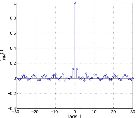
Figure 3.8 Autocorrelation of the channel noise, the large component at 0 lags suggests that the noise is approximately white with some small amount of correlation.. . . 42
Figure 3.9 Empirical relationship between SNR and measuredc(530 nm) based on linear regression. . . 50
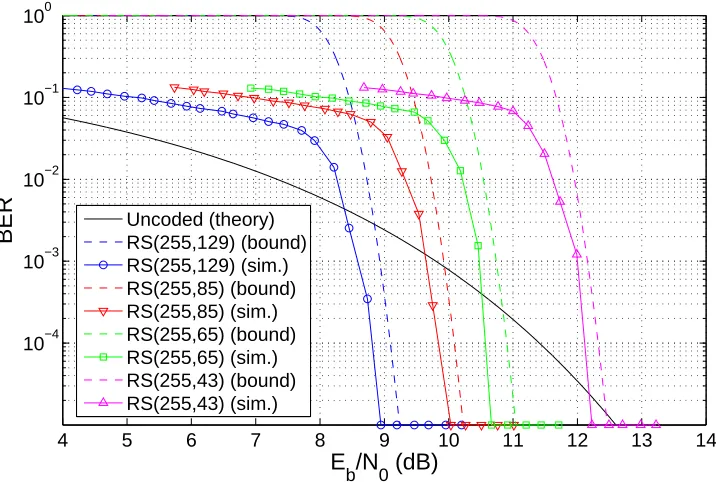
Figure 4.1 RS simulation results for codes over GF(256). . . 54
Figure 4.2 RS simulation results for codes over GF(512). . . 54
Figure 4.3 Experimental BER vs. Eb/N0 results for the CRS(255,129) code. . . 58
Figure 4.4 Experimental BER vs. da results for theCRS(255,129) code. . . 58
Figure 5.1 Turbo encoder for the UMTS turbo code. Adapted from [53]. . . 62
Figure 5.2 Simulated performance of the UMTS turbo code in AWGN using the log-MAP decoding algorithm, 16 decoding iterations, and variable frame size,k(BER vs. Eb/N0). . . 66
Figure 5.3 Simulated performance of the UMTS turbo code in AWGN using the linear-log-MAP decoding algorithm, 16 decoding iterations, and variable frame size, k (BER vs. Eb/N0). . . 67
Figure 5.4 Simulated performance of the UMTS turbo code in AWGN using the constant-log-MAP decoding algorithm, 16 decoding iterations, and variable frame size, k (BER vs. Eb/N0). . . 68
Figure 5.5 Simulated performance of the UMTS turbo code in AWGN using the max-log-MAP decoding algorithm, 16 decoding iterations, and variable frame size, k (BER vs. Eb/N0). . . 69
Figure 5.6 Experimental BER vs. Eb/N0 results for UMTS scenario 1: k = 5114, r= 1/3, log-MAP decoding, 16 decoding iterations. . . 74
Figure 5.7 Experimental BER vs.Eb/N0results for UMTS scenario 2: k= 530,r= 1/3, max-log-MAP decoding, 10 decoding iterations. . . 74
Figure 5.9 Experimental BER vs.da results for UMTS scenario 1: k= 5114,r = 1/3,
log-MAP decoding, 16 decoding iterations. . . 77 Figure 5.10 Experimental BER vs. da results for UMTS scenario 2: k = 530, r = 1/3,
max-log-MAP decoding, 10 decoding iterations. . . 77 Figure 5.11 Turbo encoder for the CCSDS turbo code. For clarity, the generators g(0)
through g(3) are labeled. Adapted from [56]. . . 79 Figure 5.12 CCSDS interleaver mapping of bits in the uninterleaved sequence to bits in
the interleaved sequence using the permutation numbers,π(s). Adapted from [56]. 82 Figure 5.13 Simulation results for CCSDS using the log-MAP decoding algorithm. . . 83 Figure 5.14 Simulation results for CCSDS using the linear-log-MAP decoding algorithm. 84 Figure 5.15 Simulation results for CCSDS using the constant-log-MAP decoding
algo-rithm. . . 85 Figure 5.16 Simulation results for CCSDS using the max-log-MAP decoding algorithm. 86 Figure 5.17 Experimental BER vs. Eb/N0 results for CCSDS scenario 1: k = 8920,
r= 1/2, log-MAP decoding, 16 decoding iterations. . . 94 Figure 5.18 Experimental BER vs. Eb/N0 results for CCSDS scenario 2: k = 8920,
r= 1/3, log-MAP decoding, 16 decoding iterations. . . 94 Figure 5.19 Experimental BER vs. Eb/N0 results for CCSDS scenario 3: k = 8920,
r= 1/4, log-MAP decoding, 16 decoding iterations. . . 95 Figure 5.20 Experimental BER vs. Eb/N0 results for CCSDS scenario 4: k = 8920,
r= 1/6, log-MAP decoding, 16 decoding iterations. . . 95 Figure 5.21 Comparison of experimental performance of the CCSDS turbo code with
information-theoretic limits. . . 96 Figure 5.22 Experimental BER vs.da results for CCSDS scenario 1: k= 8920,r= 1/2,
log-MAP decoding, 16 decoding iterations. . . 98 Figure 5.23 Experimental BER vs.da results for CCSDS scenario 2: k= 8920,r= 1/3,
log-MAP decoding, 16 decoding iterations. . . 98 Figure 5.24 Experimental BER vs.da results for CCSDS scenario 3: k= 8920,r= 1/4,
Figure 6.1 Staircase lower triangular submatrix of the DVB-S2 parity-check matrix.
Adapted from [60]. . . 105
Figure 6.2 Simulated performance of the DVB-S2 LDPC code in AWGN for normal block length (n= 64800) and 100 maximum decoding iterations (BER vs. Eb/N0).108 Figure 6.3 Simulated performance of the DVB-S2 LDPC code in AWGN for short block length (n= 16200) and 100 maximum decoding iterations (BER vs. Eb/N0). . . 109
Figure 6.4 Experimental BER vs. Eb/N0 results for DVB-S2 scenario 1: n = 64800, r= 1/2, 100 max. decoding iterations. . . 114
Figure 6.5 Experimental BER vs. Eb/N0 results for DVB-S2 scenario 2: n = 64800, r= 1/3, 100 max. decoding iterations. . . 114
Figure 6.6 Experimental BER vs. Eb/N0 results for DVB-S2 scenario 3: n = 64800, r= 1/4, 100 max. decoding iterations. . . 115
Figure 6.7 Experimental BER vs. Eb/N0 results for DVB-S2 scenario 4: n = 16200, r= 1/2, 50 max. decoding iterations. . . 115
Figure 6.8 Comparison of experimental rates vs. Eb/N0 for DVB-S2 LDPC code. . . 116
Figure 6.9 Experimental BER vs.daresults for DVB-S2 scenario 1: n= 64800,r= 1/2, 100 max. decoding iterations. . . 119
Figure 6.10 Experimental BER vs.daresults for DVB-S2 scenario 2: n= 64800,r= 1/3, 100 max. decoding iterations. . . 119
Figure 6.11 Experimental BER vs.daresults for DVB-S2 scenario 3: n= 64800,r= 1/4, 100 max. decoding iterations. . . 120
Figure 6.12 Experimental BER vs.daresults for DVB-S2 scenario 4: n= 16200,r= 1/2, 50 max. decoding iterations. . . 120
Figure 7.1 Summary of rates vs. experimentally measuredEb/N0 at BER 10−4. . . 123
Figure A.1 Plot of c(530 nm) vs. SNR and linear regression for CRS(255,129). . . 134
Figure A.3 Plot of c(530 nm) vs. SNR and linear regression for UMTS scenario 1. . . 135
Figure A.4 Plot of residuals for UMTS scenario 1. . . 135
Figure A.5 Plot of c(530 nm) vs. SNR and linear regression for UMTS scenario 2. . . 136
Figure A.6 Plot of residuals for UMTS scenario 2. . . 136
Figure A.7 Plot of c(530 nm) vs. SNR and linear regression for CCSDS scenario 1. . . . 137
Figure A.8 Plot of residuals for CCSDS scenario 1. . . 137
Figure A.9 Plot of c(530 nm) vs. SNR and linear regression for CCSDS scenario 2. . . . 138
Figure A.10Plot of residuals for CCSDS scenario 2. . . 138
Figure A.11Plot of c(530 nm) vs. SNR and linear regression for CCSDS scenario 3. . . . 139
Figure A.12Plot of residuals for CCSDS scenario 3. . . 139
Figure A.13Plot of c(530 nm) vs. SNR and linear regression for CCSDS scenario 4. . . . 140
Figure A.14Plot of residuals for CCSDS scenario 4. . . 140
Figure A.15Plot of c(530 nm) vs. SNR and linear regression for DVB-S2 scenario 1. . . . 141
Figure A.16Plot of residuals for DVB-S2 scenario 1. . . 141
Figure A.17Plot of c(530 nm) vs. SNR and linear regression for DVB-S2 scenario 2. . . . 142
Figure A.18Plot of residuals for DVB-S2 scenario 2. . . 142
Figure A.19Plot of c(530 nm) vs. SNR and linear regression for DVB-S2 scenario 3. . . . 143
Figure A.20Plot of residuals for DVB-S2 scenario 3. . . 143
Figure A.21Plot of c(530 nm) vs. SNR and linear regression for DVB-S2 scenario 4. . . . 144
Chapter 1
Introduction
In recent years, the need for high-data-rate underwater wireless communication links has increased tremendously. What began as a technological requirement primarily for military applications has expanded to include significant applications in the commercial and scientific sectors as well. A fundamental challenge in underwater wireless communication is that radio frequency (RF) links, which have enabled high-data-rate mobile communica-tion in terrestrial applicacommunica-tions, suffer such high attenuacommunica-tion under water that they can only propagate on the order of a few feet, thus making them of little use for communicating under-water. One attractive option for wireless communication in the underwater environment is
underwater free-space optical (FSO) communication, which refers to an underwater optical link, typically operating near the blue-green region of the visible spectrum, that uses water as the propagation medium (i.e., no fiber). This emerging technology shows the potential to augment existing underwater communication methods by providing high-data-rate wireless communication over short-range links.
These systems have seen significant improvement over the past three decades. However, they remain inherently bandlimited due to absorption and low operating frequencies (most systems operate below 30 kHz). They are also subject to severe multipath fading and frequency spreading due to Doppler shifts. Typical bandwidths are on the order of>100 kHz over short-range links (<100 m), 10−100 kHz over medium-range links (0.1-10 km), and <10 kHz over long-range links (>10 km) [2]. For applications in which low data rates are acceptable, underwater acoustic links are a good candidate, particularly if long-range links are desired. However, if both high data rate and mobility are required, a method other than tethered and acoustic communication is necessary.
Although it is not likely to displace underwater acoustic communication for long-range wireless links, underwater free-space optical communication is a promising new tech-nology for short-range applications, offering high data rates over distances less than 100 m. Hanson and Radic [3] demonstrated a data rate of 1 Gbps over a distance of 2 meters in a laboratory environment and used Monte Carlo simulation to suggest that data rates of 1 Gbps over a range of 48 m could be achievable in clear ocean water conditions. Chancey [4] used theoretical modeling of the underwater optical channel to suggest that data rates of >10 Mbps could be achieved over longer data links of up to 100 m, also in clear ocean water conditions. In addition to higher data rates, underwater FSO offers other advantages over acoustic communication. While underwater acoustic systems are generally broadcast in nature, underwater FSO links are typically line-of-sight and point-to-point. This property makes underwater optical systems inherently more secure and harder to intercept, which is particularly appealing in military applications where covertness is required. This property also allows for multiple links in relatively close proximity, making full-duplex communica-tion a possibility. Addicommunica-tionally, underwater optical links are not subject to the same level of multipath fading and frequency spread as underwater acoustic links, thus simplifying the digital signal processing of the receiver.
the possible applications are virtually limitless. These networks can include stationary nodes, mobile notes attached to a submarine or AUV, or a combination of both stationary and mobile nodes, as in [6]. Such sensor networks could be used for military/security purposes to monitor for underwater intruders. Terrestrial uses of wireless sensor networks include monitoring of environmental conditions including temperature change, water runoff, and pollution [7], [8]. It is certainly within reason to expect that ocean temperature, pollutants, and other measures of ecosystem health could be monitored using an underwater wireless sensor network. In particular, this technology would enable scientific observation in areas that humans and large vessels cannot easily navigate, such as deep-sea vents or underwater geological fault lines. Underwater FSO links could be an enabling technology, allowing mobile nodes in the form of AUVs to collect vast amounts of scientific data, then bring the data back to a central storage location and quickly download the data via a high-data-rate optical modem, a concept proposed in [9].
An underwater FSO link is limited by transmitter power and water turbidity. The term turbidity refers to the cloudiness or haziness of a liquid caused by suspended small particles. One well-established method of improving the performance of a communication system is through the use of forward-error correction (FEC). Forward-error correction is a method of error-control coding in which redundant bits are systematically introduced into the transmitted sequence in such a way that the receiver can correct a limited number of errors in the received message. Properly designed FEC coding schemes improve the power efficiency of a system, typically at the cost of decreased channel utilization. For an underwater FSO link, this translates into lower transmitter power requirements or extended link range. Today’s state-of-the-art FEC codes, in particular turbo codes and low-density parity-check (LDPC) codes, can achieve performance close to the optimal power efficiency dictated by information theory for a given bandwidth efficiency [10], [11]. Although the advantages of FEC have been investigated for a wide array of communication channels, little has been done so far to investigate the benefits of FEC on an underwater FSO link.
Chapter 2
Background
In this chapter we present an overview of forward-error correction. An understand-ing of this subject will be necessary in the application of FEC to the underwater optical communication channel. We begin by reviewing the fundamentals of forward-error correc-tion in Seccorrec-tion 2.1, including an introduccorrec-tion to block codes and convolucorrec-tional codes. Then we present the fundamental theory behind each of the three types of codes implemented in this thesis. This includes Reed-Solomon codes in Section 2.2, turbo codes in Section 2.3, and finally low-density parity-check (LDPC) codes in Section 2.4.
2.1
Forward-Error Correction
Communication System
Receiver Transmitter
Information Source
Source Encoder
Channel Encoder
Modulator
Source Decoder
Channel Decoder
Demodulator
Destination
Channel
u u^
c y
Noise
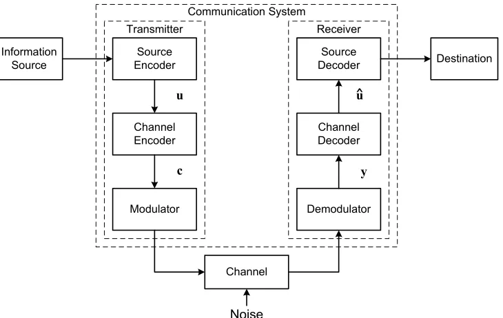
Figure 2.1: Block diagram of a typical digital communication system including forward-error correction.
channel without the use of feedback. Error detection is similar, but with the ultimate goal of detecting symbol errors in the received data sequence. For the purposes of this thesis, we are interested only in the former.
A block diagram of a typical digital communication system including FEC coding is shown in Figure 2.1. The information source can be either a person or a machine (e.g., a computer, or a data terminal). The output of the information source can be in the form of a continuous waveform or a sequence of discrete symbols. The source encoder transforms the source information into a sequence of bits called theinformation sequence,
Noise
Figure 2.2: Simplified block diagram of a coding system.
attempts to use the redundancy introduced by the channel encoder to correct errors, thus producing the estimated information sequence, uˆ. Ideally, ˆu will be an exact replica of
u; however, decoding errors may occur. Finally, the source decoder transforms ˆu into an estimate of the original information source. This estimate is then delivered at the destination.
From a coding standpoint, the system can be simplified in three ways. First, since we are only concerned with the information sequence,u, and not the form of the information source, the information source and source encoder can be reduced to a singledigital source
block. Second, the destination and source decoder can similarly be reduced to a digital sink that takes as its input the binary sequence, uˆ. Again, the context of the received information is unimportant. Third, the modulator, demodulator, and analog channel can be combined into a single block that we will call the discrete-time coding channel. The simplified block diagram of a coding system is shown in Figure 2.2. This block diagram allows us to focus on the system from an error-control coding standpoint.
The question of how to implement the channel encoder and decoder is one of the fundamental questions of error-control coding. In this section we will discuss the basic approaches to solving this problem. Most FEC codes known today fall into two main categories: Block codes and Convolutional codes (also referred to as trellis codes). These two structurally different types of codes will be introduced below.
2.1.1 Block Codes
The concept of coding data in blocks dates back to Shannon’s original 1948 work [14]. In block coding, a message block of k information symbols is uniquely mapped to n coded channel symbols, which make up a codeword. A value of particular importance is the code rate,r which is defined as
r = k
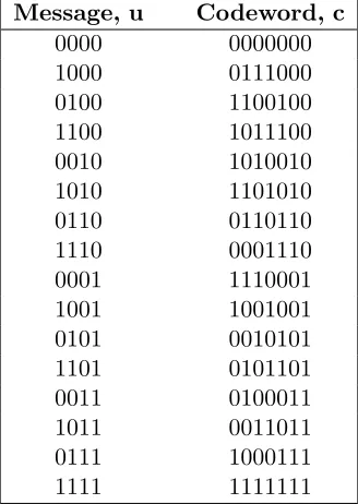
Table 2.1: The (7,4) Hamming code: a binary linear block code with k= 4 andn= 7.
Message, u Codeword, c
0000 0000000
1000 0111000
0100 1100100
1100 1011100
0010 1010010
1010 1101010
0110 0110110
1110 0001110
0001 1110001
1001 1001001
0101 0010101
1101 0101101
0011 0100011
1011 0011011
0111 1000111
1111 1111111
the fraction of information symbols to coded symbols. Typicallyk < nfor practical codes. A basic example of a linear binary block code is given in Table 2.1.
For binary block codes, one symbol corresponds to one bit and operations are performed over the binary Galois field GF(2). A Galois field, also referred to as a finite field, consists of a finite set of elements F on which two operations, addition “+” and multiplication “·”, are defined such that (F,+) and (F×,·) are each commutative groups, whereF× are all the non-zero elements inF. The binary Galois field,GF(2) consists of the elements 0,1 and the operations of modulo-2 addition and multiplication. Now, letGF(2)n
be the n-dimensional vector space over GF(2). An (n, k) binary linear block code, C, is then defined as the k-dimensional subspace of GF(2)n that is spanned by the k linearly
independent basis vectors g0,g1, . . . ,gk−1. Consider the message u = [u0, u1,· · · , uk−1] and corresponding codeword c= [c0, c1,· · · , cn−1] in codeC. The mappingu → c can be written as
G= g1 .. .
gk−1
. (2.3)
This matrix is called thegenerator matrix,G, of code C. The codewords ofC are given by all the linear combinations of rows in G. The encoding process can be viewed as a one-to-one mapping of messages in the k-dimensional message vector space onto codewords in then-dimensional vector space defined byC. Furthermore, a linear block code is said to be
systematic if the information symbols,u, appear explicitly in the codeword. In particular, if the information symbols appear at the end of the codeword then the generator matrix takes the form
G=hP Ik
i
(2.4) whereP is ak×(n−k) matrix of parity-check symbols, andIkis the k×kidentity matrix.
Since C is a subspace of the larger vector space GF(2)n, there exists a dual space
C⊥ that consists of all vectors in GF(2)n that are orthogonal to every vector in C. This
dual space is also a linear block code of dimensionn−kthat is spanned by a set of linearly independent basis vectors, sayh0,h1, . . . ,hn−k−1. The dual spaceC⊥has its own generator matrix H = h0 h1 .. .
hn−k−1
. (2.5)
This matrix is called the parity-check matrix, H, of code C. Since the dual space C⊥ is orthogonal to the code C, the multiplication of any valid codeword of C with any basis vector of C⊥ will result in the all zero vector. This leads to the following property of the parity-check matrix:
cHT =0, (2.6)
Figure 2.3: Generator and parity-check matrices for the (7,4) Hamming code.
Decoding of linear block codes is often done using minimum Hamming distance decoding. The Hamming distance between any two vectors binary x and y refers to the number of places wherexandydiffer. Consider the case where then-dimensional received vector, y, at the output of the channel is corrupted by noise. Although this vector exists withinGF(2)n, it may not exist within the subspaceCof the code. In this case, the decoder
will estimate the transmitted codewordcby the codewordˆc∈ Cthat is closest toyin terms of Hamming distance. As long as the number of errors is low enough thatyis closest to the transmitted codewordc, no error will occur in the decoded messageˆu. This concept can be visualized by recalling that each possible received vector,y, is a point in then-dimensional vector spaceGF(2)n. The codewords of C make up a subset of these points. Around each
valid codeword is a sphere such that no two spheres are overlapping. This is accomplished if the radius of the sphere is one less than half of the minimum distance between any two spheres. All points (i.e. received vectors) within a sphere are decoded as the codeword at its center. A diagram of this concept is shown in Figure 2.4.
The ability of a linear block code to correct errors is closely related to its minimum distancedmin, which is defined as the minimum Hamming distance between any two distinct
codewords of the code. A code with minimum distance dmin can correct any pattern of t
symbol errors provided that
dmin ≥2t+ 1. (2.7)
If more thant errors occur, then the received vector may be pushed out of one codeword’s “sphere” and into another, resulting in a decoding error.
Cyclic codes are a class of linear block codes which have the property that a cyclic shift of any codeword is also a codeword. This means that if c = [c0, c1,· · ·, cn−1] is any codeword of C, then c(1) = [c
t
Figure 2.4: A representation of codewords as centers of spheres of radius t = ⌊1/2 (dmin−1)⌋ in then-dimensional vector spaceGF(2)n.
logic or shift registers and because their special algebraic structure leads to more efficient decoding algorithms [15]. In addition to being expressed in vector form, cyclic codes can also be equivalently expressed as polynomials:
c= [c0, c1,· · ·, cn−1] ↔ c(x) =c0+c1x+c2x2+· · ·+cn−1xn−1 , wherex is an indeterminant variable.
In addition to the generator and parity-check matrices of regular block codes, cyclic codes can also be defined and generated by means of a generator polynomial, g(x). The generator polynomial is the unique, non-zero minimum degree code polynomial that divides all other code polynomials in the code. That is to say, any code polynomial in the code is a multiple of the code’s generator polynomial. This results in a useful encoding property of cyclic codewords. If the message is expressed in polynomial form, then the corresponding codeword can be generated by
c(x) =u(x)g(x) (2.8)
2.1.2 Convolutional Codes
Convolutional codes, which function in a manner fundamentally different than block codes, were first proposed by Elias in 1955 [16]. Convolutional encoders also createn output bits for everyk input bits; however, instead of using blocks, encoding is performed using a sliding window of data. In this case,kandnare small integers and, similar to block codes, k < n in practical codes. The encoded message now depends on both the current input message, comprised of k symbols, and m previous messages, each of which is also k symbols in length. This value, m, is the memory order of the code. For convolutional codes, redundancy is a function of the memory order of the encoder, as well as the number of parity bits in the codes. Another important parameter is the constraint length of the code, denoted by K, which is equivalent to m+ 1. For nonrecursive convolutional codes, such as the one shown in Figure 2.5 below, the constraint length indicates the maximum number of input symbols (past and present) that any of thenoutput symbols can depend on. The impulse responses of the encoder can last at mostK time units and are written as
g(ij)=hg(0ij), g1(ij),· · ·, gm(ij)i , (2.9) where g(ij) refers to the impulse response between in i-th input symbol, u
i, and the j-th
output symbol,cj. The impulse responsesg(ij)are called thegenerator sequences, or simply
thegenerators, of the encoder. In tables, the generators are often expressed in octal, with zeros padded on the left if necessary.
A simple example of a binary convolutional encoder is given in Figure 2.5. The data sequence,u, enters from the left and is stored in the binary linear shift register. Each time a new data bit arrives at the input to the encoder, the previous data bits are shifted to the right into the next flip-flop. At the output, two code bits are generated,c1i and c2i, for
D
D
D
u
ic
1ic
2iconstraint length are m= 3 andK = 4 respectively. The generator sequences, read left to right, are g(11) = 1011 and g(12)= 1111. Alternatively, the generators can be expressed in octal asg(11)= 13 andg(12)= 17. Since the input sequence does not appear at the output, this encoder is not systematic. For this reason, conventional convolutional codes of this structure are sometimes referred to asnon-systematic convolutional codes or NSC codes.
One major advantage of convolutional codes is that computationally efficient de-coding algorithms that exploit soft-decision information are known, such as the famous Viterbi algorithm [17], [18]. Since our discussion of convolutional codes is limited in appli-cation to Turbo codes, which have a very distinct decoding structure, we will not discuss the decoding of convolutional codes in detail here. However, there are a number of excellent texts on the subject, such as [15, pp. 515-738].
2.1.3 Concatenated Codes
Multiple coding schemes can be used simultaneously to improve error correction capability. In this case, two relatively small, low-complexity constituent codes are used together to create a “big code” that is more powerful than the individual codes alone. This technique is called the concatenation of codes. By breaking the encoding and decoding process into two smaller parts, concatenated codes have the advantage that they can pro-vide the same performance as a single, big code but typically at a lower cost in terms of complexity. There are basically two ways of concatenating codes: serial concatenation and
parallel concatenation.
Outer Channel Outer
Encoder (n1, k)
Inner Encoder
(n2, n1)
Inner (Physical)
Channel Inner
Decoder (n2, n1)
c
y u
u
^ Outer
Encoder (n1, k)
Figure 2.6: Structure of a serial concatenated system.
Encoder 1 u
Interleaver c
Encoder 2
c1
c2
Figure 2.7: Structure of a parallel concatenated system.
length n1 which is then decoded by the outer decoder into the received message ˆu. The structure of a serial concatenated system is shown in Figure 2.6. A widely used example of a serial concatenated code is the compact disk standard, which utilizes two shortened Reed-Solomon codes,CRS(28,24) andCRS(32,28), separated by an interleaver.
concatenation is an essential component of turbo coding systems. An understanding of the concept of parallel concatenation will be useful in our discussion of turbo codes in section 2.3.
2.2
Reed-Solomon Codes
Reed-Solomon codes are a class of non-binary cyclic block codes that were first proposed in 1960 [21]. This class of codes includes some of the most powerful known block codes, and simple decoding algorithms for these codes are known. Reed-Solomon codes are commonly used in serial concatenated systems as the outer code and are also used in computer memories and compact disc storage.
In Section 2.1.1 we focused primarily onbinary block codes. Reed-Solomon codes, however, are non-binary. This means that they are defined over the Galois field GF(q), where q > 2, rather than the binary field GF(2). An (n, k) non-binary block code over GF(q) maps k q-ary message symbols onto n q-ary code symbols. In general, q is chosen such thatq =pm wherepis any prime number. In practice, however, the most useful codes
are of the form q = 2m. Thus, a non-binary Reed-Solomon code C
RS(n, k) over GF(2m)
maps k m-bit message bytes onto n m-bit code bytes. In other words, the CRS(n, k) q-ary
code can be regarded as an equivalent (nm, km) binary code.
A Reed-Solomon code overGF(q) can be defined by its parity-check matrix, which takes on a special structure given by
H =
α1 α2 · · · αn
α12 α22 · · · α2n ..
. ... . .. ... α2t
1 α22t · · · α2nt
(2.10)
whereα1, α2,· · ·, αnare all the distinct non-zero elements ofGF(q) andtis the maximum
error correction capability of a Reed-Solomon code. All error-correcting codes must satisfy the Singleton bound, which is given by
dmin≤n−k+ 1 (2.11)
In the case of Reed-Solomon codes,dmin =n−k+ 1. Since Reed-Solomon codes achieve the
Singleton bound, they are said to bemaximum distance separable. This is a very desirable property to have in a code because it allows for the maximum number of correctable errors, t, for a given dimension,k, and block length, n.
Since Reed-Solomon codes are cyclic, they can alternatively be defined in terms of their generator polynomial. Ifα is a primitive element over GF(q), then αq−1 = 1. The CRS(n, k) code is then the cyclic linear block code generated by the polynomial
g(x) = (x−α)(x−α2)· · ·(x−αn−k) (2.12) = (x−α)(x−α2)· · ·(x−α2t) (2.13) = g0+g1x+g2x2+· · ·+g2tx2t (2.14)
where the coefficients,gi, are over the fieldGF(2m). The polynomial form of Reed-Solomon
codes is useful for systematic encoding. The systematic encoding of Reed-Solomon codes can be performed polynomial division. Letp(x) be the remainder when x2tu(x) is divided
by g(x), so
x2tu(x) =q(x)g(x) +p(x) , (2.15)
whereu(x) is the message polynomial to be encoded andq(x) is the quotient. The systematic code polynomial is formed by subtracting this remainder from the polynomialx2tu(x), i.e.,
c(x) =x2tu(x)−p(x). As an example, consider the messageu= [001 101 111 010 011]
encoded using theCRS(7,5) code that operates over the Galois fieldGF(23), generated from
the primitive polynomial pi(x) = 1 +x2 +x3. The generator polynomial for this code is
given by:
g(x) = (x−α)(x−α2) = α3+ (α+α2)x+x2
= α3+α6x+x2 . (2.16)
First the message is converted into polynomial form:
x u(x) = x u(x)
= x2 α2+α3x+α4x2+αx3+α6x4
= α2x2+α3x3+α4x4+αx5+α6x6 . (2.18) Dividing the polynomial in (2.18) by the generator polynomial, g(x), in (2.16) using poly-nomial division, we obtain the remainder:
p(x) =α5x . (2.19)
Finally, the code polynomial is formed by subtracting (2.19) from (2.18), which gives c(x) =α5x+α2x2+α3x3+α4x4+αx5+α6x6 , (2.20) which in equivalent vector form is equal toc= [000 110 001 101 111 010 011]. This form is clearly systematic, as the original message, u appears in the last five 3-bit bytes, i.e., the lastmk= 15 bits, of the codeword.
As mentioned above, there are several known efficient algorithms for the decoding of Reed-Solomon codes. Notable amongst these is the Berlekamp-Massey-Forney algorithm [22, pp. 128-136], which we will utilize in our implementation of a Reed-Solomon coded system in Chapter 4.
2.3
Turbo Codes
Upper Encoder
u
iInterleaver
Lower Encoder
z
iz'
i InterleavedParity Uninterleaved
Parity
Systematic Output
u
iMultiplex and Puncture
c
Figure 2.8: General structure of a turbo encoder.
2.3.1 Turbo Encoder
The turbo encoder consists of two parallel concatenated, systematic encoders sepa-rated by an interleaver. In general, the systematic bits of the second encoder are suppressed, as they are just a reordering of the systematic bits of the first encoder. A diagram of a generic turbo encoder is shown in Figure 2.8. The parity bits of the upper encoder are denoted zi and those of the lower encoder are denoted zi′. Although almost any type of
encoder could be used for the constituent encoders, in practice they are almost always re-cursive systematic convolutional (RSC) encoders. The RSC encoders are similar in nature to the non-systematic convolutional (NSC) encoders described in Section 2.1.2. Fork= 1, an RSC encoder can be created from an NSC encoder by feeding one of the two coded out-puts back to the input of the encoder. It is this feedback structure that makes it recursive. An example of a rate r = 1/2 RSC encoder is given in Figure 2.9. Although the two con-stituent encoders can be different (asymmetric), they are typically the same (symmetric) in practice [23].
D
D
D
u
iFigure 2.9: Example of a rate 1/2 recursive systematic convolutional (RSC) encoder.
be of the form c = [u0, z0, z′0, u2, z0, z1′,· · ·]. In order to raise the code rate to r = 1/2, the output can drop every odd bit parity bit of the lower encoder and every even bit of the upper encoder. The codeword will then be of the form c = [u0, z0, u1, z1′, u2, z2,· · ·]. This process of systematically dropping coded bits to increase code rate is referred to as
puncturing.
Although the convolutional encoders can encode data in a continuous stream, in practice it is desirable to break up encoded data into discrete chunks calledframes. At the end of a frame, the output of the encoders is forced back to the all-zero sequence. Unlike NSC encoders, RSC encoders have an infinite impulse response due to their recursive structure. As such, they cannot in general be forced back to the all-zero state by simply inserting a string of zeros at the input. Thus, in order to end a frame and reinitialize the RSC encoders to the all-zero state, a zero-forcing sequence is needed. The feedback data provides such a sequence. Thus, an RSC encoder can be forced back to the all-zero state by connecting the feedback path directly to the input of the encoder for m time shifts.
The interleaver1 at the input of the second constituent code is an essential com-ponent of a turbo code that has a major influence on BER performance. The interleaver rearranges a block of data in a prescribed, but irregular pattern. Because the pattern is prescribed, a corresponding deinterleaver can restore the original order of the data at the receiver. By changing the order of the data bits in a pseudo-random way, the interleaver ensures that the input to each constituent encoder is different, resulting in different parity
1It is important to differentiate turbo code interleavers from the rectangular interleavers used in wireless
bits at the output of each. In addition to the property of being pseudo-random, the size of an interleaver has a significant impact on its performance. Longer interleavers result in enhanced BER performance of the turbo code, but this comes at the cost of increased delay in the system, which may not be desirable in some applications [23].
2.3.2 Turbo Decoder
Another element that is essential to the performance of turbo codes is iterative soft-input, soft-output (SISO) decoding. A diagram of a turbo decoder is shown in Fig-ure 2.10. The overall structFig-ure of the turbo decoder is built around two processors that share information. One processor operates on information from the parity bits of the upper constituent encoder, while the second processor operates on information from the parity bits of the lower constituent encoder. During each iteration, the upper processor uses a priori probabilities of the data sequence to calculate a posteriori probabilities of the data sequence. Thesea posteriori probabilities are then used to form the inputa priori probabil-ities to the lower processor which, in turn, calculates its own set ofa posteriori probabilities. The output of the lower processor is then used to form the input to the upper processor for the next iteration. It is this exchange of information back and forth that makes the decoder iterative. Each iteration improves the decoder’s ability to estimate the transmitted sequence. After each iteration, the decoder is better able to estimate the decoded sequence, although each iteration yields diminishing returns. Turbo codes derive their name from this iterative decoding structure which resembles the feedback system between the exhaust and the intake compressor in a turbo engine.
To better understand how the turbo decoder works, we now follow the flow of data in Figure 2.10. Let ci represent a coded data bit, either systematic or parity, at the input
of the channel and let yi represent the corresponding received signal (i.e., the output of a
correlator or matched filter receiver). Sinceci can only be a 1 or a 0, it is said to be ahard value. However, if the received signal is left unquantized or quantized to more than one bit, the received symbol,yi, can take on a larger range of values. In this case,yi is said to be a soft value. The input to the turbo decoder is a probability measure in log-likelihood ratio (LLR) form,
R(ci) = ln
P(yi|ci= 1)
P(yi|ci= 0)
Convert to LLR
form
y R(zi)
R(z’i)
SISO Processor
Lower SISO Processor Interleaver
Deinterleaver
Λ2(u’i)
Λ2(ui)
V2(ui)
V2(u’i)
u
^
-Figure 2.10: Structure of a turbo decoder. Adapted from [23].
where P(yi|ci = b) is the conditional probability of receiving yi given that ci = b was
transmitted. Note that these are soft values. One advantage of using LLRs is that a hard decision can be made by taking the sign of the value. On the other hand, the magnitude of the value reflects the amount of certainty that the value is a 0 or 1. Additionally, calculations of Equation 2.21 require some knowledge of the channel characteristics.
At the input of the turbo decoder, LLRs are calculated separately for the system-atic and parity bits, denotedR(ui),R(zi), andR(z′i). The upper processor takesV1(ui) and
R(zi) as its systematic and parity inputs, respectively. For the first iteration, the systematic
input, V1(ui), is simply equal to R(ui). The upper processor then computes a posteriori
LLR value for each data bit of the form Λ1(ui) = ln
P(ui = 1|y)
P(ui = 0|y)
(2.22) where y = [y1, y2,· · · , yn] is the received sequence corresponding to the entire encoded
frame. For the first iteration, this value Λ1(ui) is simply interleaved to form the systematic
input to the second encoder, denoted V2(u′i). The second processor then uses V2(u′i) along
with the parity input from the lower constituent encoder,R(zi′), to compute a similar LLR estimate, Λ2(u′i). This value is then deinterleaved and fed back into the first processor for
it is important to avoid positive feedback, which would result in an unstable system. To ensure that only information which is unique to a given decoder iteration is fed back, the input of each processor is subtracted from its output prior to feeding information to the other processor. This difference value is called the extrinsic information and is denoted by w(ui) [23, pp. 387-388]. In subsequent iterations the systematic inputs to the upper and
lower encoders are formed as
V1(ui) = R(ui)−w(ui), (2.23)
V2(ui) = Λ1(ui)−w(ui). (2.24)
Once the desired number of iterations have been completed, a threshold is used to obtain a hard decision on the decoded message, ˆu
Both of the processors within the decoder take soft LLR values as inputs and produce similar values at their output. For this reason they are referred to as soft-input, soft-output (SISO) processors. The traditional Viterbi algorithm, commonly used to decode convolutional codes, cannot be used in these processors because it generates a hard output. Instead, a SISO algorithm must be used. Two commonly used algorithms are the soft-output Viterbi algorithm (SOVA) [24] and the maximum a posteriori (MAP) algorithm (also known as the Bahl-Cocke-Jelinek-Ravive (BCJR) algorithm) [25]. In general, the BCJR algorithm outperforms the SOVA algorithm in iterative decoders, though it is more complex. In order to reduce complexity, the MAP algorithm can be implemented in the log domain, which reduces complexity by changing multiplications to additions. This algorithm is called the log-MAP algorithm [26]. One downside to this approach is that the addition of two variables,x and y, is transformed into the operation
ln(ex+ey) (2.25)
which is difficult to compute. Simplifications to this algorithm were developed by Viterbi in [26]. Consider the functionmax-star defined as:
max∗(x, y) = ln(ex+ey) (2.26)
= max(x, y) + ln(1 +e−|y−x|) (2.27) = max(x, y) +fc(|y−x|) (2.28)
wherefc(x) = ln(1 +e−x). Rather than calculating the exact value offc, an approximation
constant-log-MAP algorithm. Third, the simplest approximation is to setfc = 0, such that
max∗(x, y) =max(x, y). This algorithm is called the max-log-MAP algorithm, and is the least computationally intensive simplification.
2.4
Low-Density Parity-Check Codes
Low-density parity-check (LDPC) codes were originally presented by Gallager in 1962 [28, 29]. Despite their excellent performance, LDPC codes were not considered by the coding community. This was primarily due to the fact that the iterative decoding method proposed by Gallager was too computationally intensive for the technology available at that time. In 1996, after the discovery of turbo codes, LDPC codes were rediscovered by MacKay and Neal [30]. Today LDPC codes are recognized as one of the most powerful state-of-the-art coding schemes known. They are Shannon limit approaching codes capable of achieving performance as good as – and, in some cases, better than – turbo codes.
2.4.1 Structure and Classification of LDPC Codes
lengths on the order of 104 bits. For these codes, certain structures must necessarily be imposed on the H matrix to both facilitate the description of codes and reduce encoding complexity. These structures will be discussed in a standard-specific context in Chapter 6.
2.4.2 Decoding LDPC Codes: The Sum-Product Algorithm
The decoding of LDPC codes is done using an iterative algorithm that uses soft-bit information similar to that of the turbo decoder. The best known algorithm for decoding LDPC codes is thesum-product algorithm, also known as iterative probabilistic decoding or
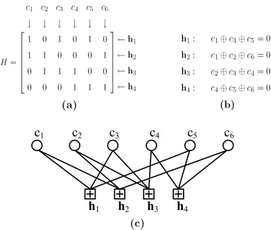
belief propagation [32]. In order to demonstrate this algorithm, it is helpful to first define a graphical representation for linear block codes called a Tanner graph [33]. An example parity-check matrix, its parity-check equations, and its corresponding Tanner graph are shown in Figure 2.11. The Tanner graph consists of two types of nodes,bit nodes andcheck nodes, which are connected by edges. The bit nodes represent then bits of the codeword. The check nodes represent the n−k parity-check equations, hi. A bit node is connected
to a check node by an edge if and only if the corresponding code bit is contained in the corresponding parity-check equation. Since edges between any two nodes of the same type are not allowed, the Tanner graph is said to be bipartite. If there are d edges emanating from a node, the node is said to be of degree d. Let us also define a cycle as a series of edges, each traversed only once, that start and end at the same bit node. In decoding via the sum-product algorithm, it is desirable to avoid short cycles of length 4 and, to a lesser extent, length 6. This is because short cycles limit decoding performance and can prevent the algorithm from converging to the maximum likelihood decision value [15, p. 858].
With an understanding of Tanner graphs, it is now possible to summarize the iterative decoding of LDPC codes based on the sum-product algorithm. The objective is to find the most likely received codeword,ˆc, such thatˆcHT =0. To do so, we will employ two values,Qx
ij and Rxij, where:
• Qx
ij is the probability that thej-th bit ofˆchas value x, wherex∈0,1, given
informa-tion obtained from all parity-check nodes connected tocj other than hi. This value
is passed from bit node tocj to check node hi.
• Rx
ij is the probability that thei-th parity-check equation,hi, is satisfied ifcj is fixed
h
1c
2c
3c
4c
5h
2h
3h
4c
6c
1Figure 2.11: The Tanner graph is a way of representing a parity-check matrix graphically. Depicted are (a) an example parity-check matrix, (b) its parity-check equations, and (c) the corresponding Tanner graph.
given by the probabilitiesQx
ij. This value is passed from check node hi to bit nodecj.
The algorithm begins with an initialization to determine the initial values of Qx
ij. In this
step,Qx
ij are set to the estimates of the received symbols, denoted fjx, the probability that
the j-th symbol is x given the received symbol yj. For the AWGN channel with on-off
keying (OOK), these values are:
fj0 = √1 2πσe
−yj2
2σ2 (2.29)
fj1 = √1 2πσe
−(yj−1)2
R
21. . .
h
2c
1c
2c
6c
7Q
22Q
26Q
27R
xQ
xQ
xQ
xFigure 2.12: Horizontal step of the sum-product algorithm.
Horizontal Step
The next step is referred to as thehorizontal step, because it operates across each row of the H matrix. In this step, each check node, hi, is inspected and, for each edge
connected tohi, two values are computed: R0ij and R1ij. The probability thathi is satisfied
given cj =x is given by
P(hi|cj =x) =
X
ˆ c:cj=x
P(hi|ˆc)P(ˆc|cj =x) (2.31)
whereP(hi|ˆc) is equal to 1 if the parity-check equationhi is satisfied or 0 if it is not satisfied.
The values ofRx
ij are now calculated as
Rijx = X ˆ c:cj=x
P(hi|ˆc)
Y
k∈N(i)|j
Qck
ik (2.32)
where N(i)|j represents all the indexes of the bit nodes connected to check node hi with
the exclusion ofcj. As an example, consider an LDPC code with parity-check equationh2 defined asc1⊕c2⊕c6⊕c7 = 0. The corresponding values ofR021and R121passed from check node h2 to bit nodec1 are thus given by:
R021 = Q022Q026Q027+Q122Q126Q270 +Q122Q026Q127+Q022Q126Q127 (2.33) R121 = Q122Q026Q027+Q022Q126Q270 +Q022Q026Q127+Q122Q126Q127 (2.34)
R
41h
2Q
22h
3h
4R
31R
xR
xQ
xFigure 2.13: Vertical step of the sum-product algorithm.
Vertical Step
The next step is referred to as the vertical step, because it operates across each column of the H matrix. In this step, each bit node receives the values of Rx
ij from its
adjacent check nodes and then updates the values of Q0ij and Q1ij. This is done using the equation
Qxij =αijfjx
Y
k∈M(j)|i
Rxkj (2.35)
where M(j)|i represents the indexes of all check nodes connected to bit node cj with the
exclusion ofhi. The variableαij is a normalization factor chosen such thatQ0ij +Q1ij = 1.
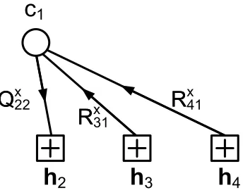
As an example, consider an LDPC code in which the code bit,c1, participates in 3 parity-check equations, denoted h2, h3, and h4. In this case, the updated values ofQ021 and Q121 to be passed from bit nodec1 check nodeh2 in the next iteration are given by
Q021 = α21f10R310 R041 (2.36) Q121 = α21f11R311 R141 (2.37) and the correction factor is
α21=
1
f10R031R041+f11R131R141. (2.38) This process of updating an edge as part of the vertical step is illustrated in Figure 2.13.
After each horizontal step, an estimate of ˆc can be calculated for that iteration. Each bit estimate, ˆcj, is chosen based on the larger a posteriori probability measure, i.e.
ˆ
cj = arg maxxfjx
Y
k∈M(j)
whereM(j) are the indexes of all the parity nodes connected to bit node cj. At this point
the algorithm computes the valueˆcHT and does one of three things:
1. If the algorithm has converged upon a codeword, i.e. ˆcHT = 0, then the algorithm
stops and decodesuˆ fromˆc.
2. If the algorithm has not converged upon a codeword, i.e. ˆcHT 6=0, and the maximum
number of iterations have not been met, then the algorithm proceeds to the vertical step for another iteration.
3. If the algorithm has not converged upon a codeword, and the maximum number of iterations have been met, then a decoding failure has occurred. In this case the algorithm returns the error codewordˆc and flags it as a decoding error.
Chapter 3
Channel Characterization and
Estimation
In this chapter we will explore light propagation and noise statistics in an underwa-ter free-space optical (FSO) communication channel testbed in order to establish a channel model for theoretical studies. Since signal-to-noise ratio (SNR) estimation is important in practical analysis, an SNR estimator is established as well. This chapter is structured as follows. In Section 3.1 a brief discussion of the propagation of light through water and Beer’s Law is presented. In Section 3.2, the underwater free-space optical communication testbed and experimental procedure are described. Then, in Section 3.3, experimental re-sults obtained on the experimental testbed are used to characterize the channel noise and a mathematical model for the underwater FSO channel is developed. A maximum-likelihood SNR estimator is established in Section 3.4. Finally, in Section 3.5, Beer’s Law is used to establish a link between coding gains in electrical SNR and range extension of a FEC-coded system.
3.1
Propagation of Light through Water
sys-Figure 3.1: Attenuation of electromagnetic radiation in seawater. Reproduced from [34].
tems, suffer a large attenuation allowing them to propagate only a few feet underwater. At infrared frequencies (∼300 GHz - 400 THz), which are typically used in fiber optic systems, attenuation is even greater. There is however a “window” of transmission through seawa-ter in approximately the blue-green region of the optical spectrum. This corresponds to a frequency of around 625 THz or a wavelength of around 480 nm. The low attenuation in this region makes underwater free-space optical communication in the blue-green spectrum a good option for wireless communication underwater.
of water are those which are a function only of the material properties of the medium itself, independent of the properties of the light source. The apparent optical properties, on the other hand, are those which depend on both the geometrical structure of the light field and the inherent optical properties of the medium. Inherent optical properties include, most notably, absorption, scattering, and attenuation, while apparent optical properties include radiometric quantities such as irradiance reflectance, radiance reflectance, and attenuation coefficients for upwelling and downwelling irradiance [36].
To understand the underwater FSO communication channel, the inherent optical properties of spectral absorption and spectral scattering are the most significant, since they are the main source of signal attenuation [37]. Seawater is a complex mixture of dissolved substances, organic matter, living organisms, and water molecules themselves, all of which contribute to its optical properties. Table 3.1 summarizes the contribution of the main components of seawater to spectral absorption and spectral scattering and their corresponding dependence on wavelength (denoted byλ).
3.1.1 Absorption
32 Table 3.1: Summary of absorption and scattering characteristics of seawater. Adapted from [38].
Absorption Scattering
Characteristic λdependence Characteristic λdependence
Water Invariant at constant
temp. and pressure strong
Invariant, small compared to
absorption
λ−4
Sea salts (inorganic)
Negligible in visible spectrum
Some increase
towards shortλ Appreciable None
Colored dissolved organic matter (yellow substance)
Variable Increase towards
shortλ None None
Particulate matter (including
phyto-plankton and detritus)
Variable Increase towards
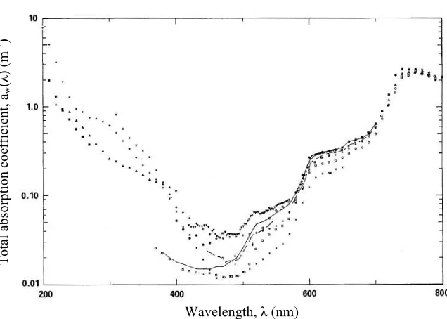
ton [36, 38]. CDOM, also referred to as yellow substance or Gelbstoff, is a rather loosely defined combination of chemical compounds resulting from the decomposition of marine organisms. According to Shifrin [39], about 150 different organic substances have been identified and there are likely more that have not been identified. Absorption by CDOM decreases with wavelength and usually dominates seawater absorption forλ <400 nm [36]. Another major organic contributor to spectral absorption is phytoplankton, microscopic plants that exist in suspension in many types of seawater. Absorption by phytoplankton is primarily due to pigments within phytoplankton cells. These pigments, generally referred to aschlorophyll, include chlorophyll a and accessory pigments such as pheophytina. The absorption spectrum of phytoplankton cells includes a strong absorption band in the blue (λ= 440 nm) attributed to accessory pigments, and a weaker absorption band in the red (λ = 675 nm) attributed to chlorophyll a [36]. Absorption due to phytoplankton varies based on concentration, with higher concentrations near the surface. The third major or-ganic contributor to spectral absorption is detritus, oror-ganic waste formed by dead plants and animals and fecal material. Having similar origins to CDOM, detritus displays a similar absorption spectrum to CDOM with absorption decreasing with wavelength at the lower boundary of the blue-green window [36].
The absorption of seawater is given by the spectral absorption coefficient, a(λ). This value is calculated as the sum of the above factors, i.e.
a(λ) =aw(λ) +aCDOM(λ) +aphy(λ) +adet(λ) (3.1)
where aw(λ) is absorption due to pure seawater, aCDOM(λ) is absorption due to CDOM,
aphy(λ) is absorption due to phytoplankton, and adet(λ) is absorption due to detritus (cf.
Wavelength, λ (nm)
T
o
ta
l
ab
so
rp
ti
o
n
c
o
ef
fi
ci
en
t,
aw
(λ
)
(m
-1 )
Figure 3.2: Absorption of pure seawater as a function of wavelength as given by multiple studies. Adapted from [40].
3.1.2 Scattering
Scattering is the process in which light energy in the form of a photon is redirected spatially from the forward propagating path due to interaction with molecules or particles. Unlike absorption, the photon is not converted to another form of energy in a scattering event [35]. Scattering can be divided into two types: Rayleigh scattering, which occurs for small particles with radiusr << λ, and Mie scattering, which occurs for larger particles with radiusr ≈λand larger. A fundamental difference between these two types of scattering is that Rayleigh scattering tends to scatter uniformly in all directions while Mie scattering is biased in the forward direction [41].
value is calculated similarly to the spectral absorption coefficient:
b(λ) =bw(λ) +bphy(λ) +bdet(λ) (3.2)
wherebw(λ) is scattering due to pure seawater, bphy(λ) is scattering due to phytoplankton,
and bdet(λ) is scattering due to detritus (cf. [36, p. 143]).
3.1.3 Attenuation
Attenuation of an optical signal transmitted through water is primarily caused by absorption and scattering, as described above. The attenuation of seawater is quantified by the spectral attenuation coefficient,c(λ). This value is defined as as the sum of the spectral absorption and spectral scattering coefficients, i.e.
c(λ) =a(λ) +b(λ) . (3.3)
In practice, c(λ) is typically measured with a transmissometer consisting of a calibrated, stable light source and a narrow field-of-view detector separated by a small distance. The attenuation of an optical signal as a function ofc(λ) and distance, d, is described by Beer’s Law:
I =I0e−c(λ)d (3.4)
whereI is the detected intensity at the receiver, I0 is the transmitted intensity, c(λ) is the spectral attenuation coefficient as a function of wavelength, anddis optical path length in meters [41].
more prevalent, while in pure seawater Beer’s Law is more directly applicable. In this work, Beer’s Law is assumed to hold for simplicity. However, it should be noted that it is unclear whether results measured in the lab can be directly extrapolated to longer distances and a wider range of water conditions.
3.2
Experimental Setup and Procedure
3.2.1 System Architecture
The experimental results in this thesis were obtained using an underwater testbed developed by Cox and Simpson in [12] and [13]. The system consists of a laser-diode-based transmitter and a photodiode laser-diode-based receiver operating through a custom-built 3,800 liter indoor water tank. The purpose of the underwater testbed is to simulate a practical underwater communication environment by emulating a range of controlled underwater scenarios. An overview of the system architecture is included for completeness but is not a novel contribution of this thesis. A more detailed description of the system architecture can be found in [44].
The laser-diode-based transmitter employs intensity modulation (IM) using on-off keying (OOK) and return-to-zero (RZ) line coding with a 50% duty cycle to transmit at a baud rate of 500 kbps. The light source is a 405 nm (blue) indium-gallium-nitride laser-diode operating at a laser power of 100 mW. This setup offers moderately high optical power and falls within the blue-green window discussed in Section 3.1. No optical attenuator is used at the transmitter. Rather, the attenuation of the transmitted signal is entirely due to the channel medium itself. The data packets to be transmitted originate from the transmitter personal computer (PC). There the data are generated, encoded, and packetized using MATLAB. The details of the packet structure are discussed below. The data packet is then streamed via USB to an FPGA board which buffers the data and sends them to the laser-diode driver.
Matched Filter
Down-sample
Symbol Sync. Remove
Header & Unpad FEC
Decoder BER
Tester
SNR Estimator
From Rx PC Post-processing
Figure 3.3: MATLAB processing architecture.
8-bit analog-to-digital converter (ADC). The ADC samples the signal at a rate of 10 MSps, resulting in 20 times oversampling of the OOK modulated signal. An FPGA board buffers the data until the entire packet is received and then transmits the received data to the PC via USB for post-processing in MATLAB.
The underwater FSO channel is emulated by means of an indoor water tank con-structed out of wood and fiberglass. The tank is 3.66 m long, 1.2 m wide, and 1.2 m tall and is capable of holding 3,800 liters of water. Polycarbonate viewing windows are installed on the long ends of the tank for the transmitter and receiver. The transmitter window is circular, 20 cm in diameter, and the receiver window is rectangular, 53 cm high and 38 cm wide. Different water conditions are simulated by varying the concentration of a scattering agent (Maalox) consisting of suspended particles.
![Figure 2.10: Structure of a turbo decoder. Adapted from [23].](https://thumb-us.123doks.com/thumbv2/123dok_us/1467455.1179791/37.612.110.540.106.322/figure-structure-turbo-decoder-adapted.webp)
![Figure 3.1: Attenuation of electromagnetic radiation in seawater. Reproduced from [34].](https://thumb-us.123doks.com/thumbv2/123dok_us/1467455.1179791/46.612.171.478.110.345/figure-attenuation-electromagnetic-radiation-seawater-reproduced.webp)