Comparative Study of Optimal Power Flow with Different Methods

(1)

Research Development Cell, Government College of Engineering, Jalagon (M. S), India

Comparative Study of Optimal Power Flow

with Different Methods

Nilesh Rajurkar1, Prashant Beddekar2

P.G. Student, Department of Electrical Engineering, GCOE, Amravati, Maharashtra, India1

Associate Professor, Department of Electrical Engineering, GCOE, Amravati, Maharashtra, India2

ABSTRACT: In this paper four different techniques conventional method, Sequential Quadratic Programing(SQP), Genetic Algorithm (GA),multiobjective Genetic Algorithm (MGA)are used to find optimal power flow solutions of an electrical power system.The power flow constraint of the power generators are included in optimal power flow problem in addition to the conventional constraint. Cost of power generated is minimized with objective function minimization and validity of their efficiency is checked with the help of different methods. Given methods are tested on IEEE standard 30 bus system.

KEYWORDS: SQP, GA, MGA, Optimal Power flow

I. INTRODUCTION

Moving towards the competitive environment pushes the power transmission systems closer to their stability limits. Thus there is a need to provide optimal power to improve the efficiency and reduce the operating costs. This trend results in several voltage collapse events which brought up the stability as a major concern in optimal power flow (OPF) problem. The overall stability limit can be modelled by voltage stability margin defining critical loading point but in reality the stability problem appears to be an OPF-like problem, in which stability can be viewed as a constraint in addition to the normal OPF voltage constraints, therefor first thestudy of OPF is important. Often trial and error used that can be costly and imprecise, hence new methodologiesare used that eliminates the need for repeated simulation and saves time and effort.First we will see different popular methods used previously; Comparative study of GA and Particle Swarm Optimization (PSO) [10], Interline Power Flow Controller (IPFC) [11],Modified cataclysmic genetic algorithm [12], artificial bee colony algorithm [13]. Simulations results are obtained on standard IEEE 30-bus system for minimizing the operating cost of generation and optimal parameters are calculated.

The organization of the paper is as follows: Section II explains OPF problem objective function, equality and inequality constraints; Section III describes the detail of conventional method and algorithm to solve optimization problems, SQP is discussed in Section IV; Section V describes the Genetic Algorithm and Modified Genetic Algorithm procedure to solve optimization problems. A comparison of simulation results obtained using conventional method, SQP, GA and MGA for IEEE 30-bus system is presented in Section VI. Section VII describe conclusion.

II. PROBLEM FORMULATION

In general, the optimal power flow problem is formulated as an optimization problem in which a particular objective function is minimized while satisfying a number of equality and inequality constraints. The main objectives of the OPF problem are taken into consideration here is minimization of fuel cost in the normal state and the minimization of the fuel cost when generator limits are given. Objective function is given as.

(2)

Research Development Cell, Government College of Engineering, Jalagon (M. S), India

Equality constraints are power flow equations of the problem, while the inequality constraints include the limits on real power generation of each plant as follows

Equality constrains

( )− ≤ (2)

Inequality constrains

≤ ≤ , =1,2, … (3) Where,

F is function to be minimize

is cost function of ith generator bus

is active power generated by each generating plant is number of generator buses

is total power demand

is tolerance limit (0.001 for programming purpose)

The equality constraints given by the above equations are satisfied by running the power flow program.

III.CONVENTIONAL METHOD

Hadi Saadat in his book [9] explains the conventional method for calculation of optimal power flow by iterative method using Lagrange multipliers. In this method objective function is modified by adding in product with equality constrains as follows

ℒ= + − (4)

Where,

ℒ is modified objective function

incremental cost of generation ($/MWh)

Minimum of this objective function is found by equating its partial derivative with respect to its variable i.e. to zero

ℒ

= 0

+ (0−1)

Since,

= + + +. …

Then,

= =

Hence condition for optimal dispatch becomes,

= = 1,2, . . (5)

And hence

+ 2 =

therefore

= −

(3)

Research Development Cell, Government College of Engineering, Jalagon (M. S), India

But

= (7)

=

+∑

∑ (8)

∆ = − (9)

= +∆ (10) Where,

∆ = ∆

∑ (11)

1. Algorithm

Step 1: assume initial value of equal to or more than largest value of Step 2: calculate value of from equation (6)

Step 3: calculate ∆ and equate it to , if ∆ ≤ ,then check generator limits

≤ ≤ , then optimal solution obtained, goto step 6

≤ , then = for rest of iteration, continue

≤ , then = for rest of iteration, continue If ∆ > , then continue to next step

Step 4: calculate ∆ and from equation (10) and (11). Step 5: repeat from step 2.

Step 6: exit.

IV.SEQUENTIAL QUADRATIC PROGRAMMING

1. General information

SQP stands for Sequential Quadratic Programming, this method invented in the mid-seventies, SQP can be viewed as the Newton approach applied to the optimality conditions of the optimization problem. Each iteration of the SQP algorithm needs finding a solution to a quadratic program (QP). This is a simpler optimization problem, which has a quadratic objective and linear constraints. QP is still difficult to solve however, it is hard when the quadratic objective is nonconvex. On the other hand, as a Newton method, the SQP algorithm converges very rapidly, means it requires few iterations (hence QP solves) to find an approximate solution with a good precision (this is particularly true when second derivatives are used). Therefore, one can say thatthe SQP algorithm is an appropriate approach when the evaluation of the functions defining the nonlinear optimization problem, and their derivatives, is time consuming.

2. Algorithm accessing toolbox

Step 1: make a function file in MATLAB with objective function. Step 2: make script file with constrained.

Step 3: open optimization toolbox and enter objective function, limits,constrains. Step 4: run

V. GENETIC ALGORITHM AND MULTI OBJECTIVE GENETIC ALGORITHM

1. History and working principle

(4)

Research Development Cell, Government College of Engineering, Jalagon (M. S), India

came up with the publication of David Goldberg’s 1989 book [10]. The publication of Goldberg’s text accelerated the application of GA. Since then, search algorithms from GA have been applied in a diverse array of disciplines, and the benefits resulting from these efforts have been numerous.

The GA Algorithm works by creating an initial population of N possible solutions in the form of candidate chromosomes. Each of these individuals is a representation of the target system. Initial population could be generated at random, or as genetic material from some previous procedure. A population consists of a collection of chromosomes. Every chromosome represents a possible solution. Each chromosome consists of one or more genomes. A particular feature in the chromosome is represented by a genome. The nature of a genome depends on the underlying data representation. For binary representations, the genome is a series of bits. For a real number representation, the genome is an integer or floating-point number.

Multi-objective optimization has been applied in many fields of science, including engineering, economics and logistics (see the section on applications for detailed examples) where optimal decisions need to be taken in the presence of trade-offs between two or more conflicting objectives.‘gamultiobj’ can be used to solve multi objective optimization problem in several variables. Here we want to minimize two objectives, each having one decision variable.

min ( ) = [ 1( ); 2( )]

2. Algorithm accessing toolbox

Step 1: make a function file in MATLAB with objective function. Step 2: make script file with constrained.

Step 3: open optimization toolbox and enter objective function, limits. Step 4: run

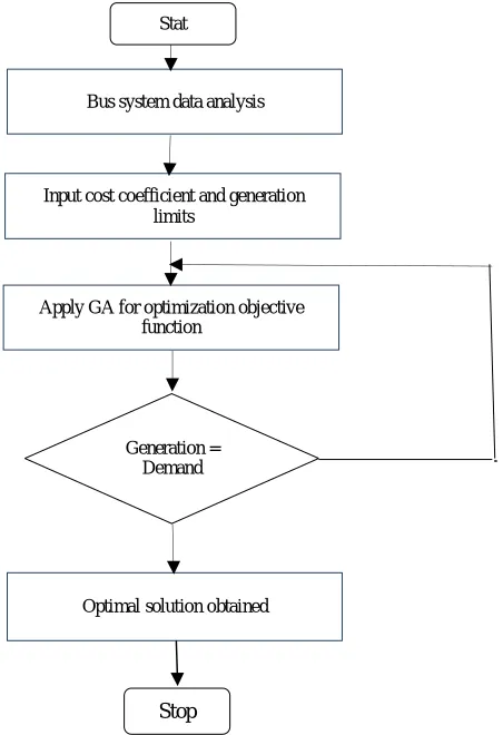
Fig. 2 Flow chart of execution of GA

Generation = Demand

Optimal solution obtained

Stop

Input cost coefficient and generation limits

Bus system data analysis Stat

(5)

Research Development Cell, Government College of Engineering, Jalagon (M. S), India

VI. RESULT

The proposed solution techniques were applied in several test cases yielding good results. The program was written in Matlab R2015a.To illustrate the efficiency of the algorithmperformance of the conventional method, SQP, GA, MGA tested on IEEE 30 bus and results were obtained. In given bus system there are 6 generator bus, 25 load buses, 41 transmission line. Cost coefficients and generator limits are given Table 1, total load demand of system is 283.4 MW

Table 1

Generator data for 30 bus IEEE test system Bus no

MW MW

Cost coefficient

a B c

1 50 200 0 2.0 0.00375

2 20 80 0 1.75 0.01750

5 15 50 0 1.0 0.06250

8 10 35 0 3.25 0.00864

11 10 30 0 3.0 0.02500

13 12 40 0 3.0 0.02500

1. Results with conventional method

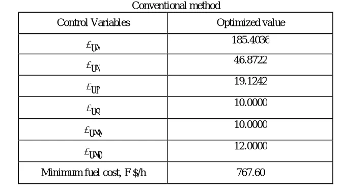
Table 2 shows the optimization results for conventional method, it gives optimized active power generation by each generator and optimal cost of generation. For initial value of is should be chosen equal to or greater than largest value among coefficient b. Iterations are taken until absolute value of ∆ > . For this above example 18 iterations were needed.

Table 2 Conventional method

Control Variables Optimized value

185.4036

46.8722

19.1242

10.0000

12.0000

Minimum fuel cost, F $/h 767.60

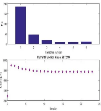
2. SQP result

(6)

Research Development Cell, Government College of Engineering, Jalagon (M. S), India

Fig. 1 Shows optimized power generation values and cost at each iteration

Table 3 SQP method

185.403

46.872

19.124

10

12

3. Genetic algorithm result

(7)

Research Development Cell, Government College of Engineering, Jalagon (M. S), India

Table 4

Genetic algorithm method

185.942

46.228

19.045

10..063

10.120

12.000

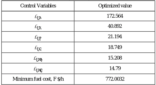
4. Multi objective genetic algorithm

Table 5 gives results for optimization with the help of multiobjective genetic algorithm. It gives different results comparing to other method.

Table 5

Multiobjective genetic algorithm method

172.564

40.892

21.194

18.749

15.208

14.79

Finally results of all methods are combined and presented in Table no. 6.

Table 6

Comparative analysis of all method

Control Variables

Optimized value

Conventional method SQP GA MGA

185.4036 _185.403 _185.942 _172.564

(8)

Research Development Cell, Government College of Engineering, Jalagon (M. S), India

10.0000 10 10.120 15.208 12.0000 12 12.000 14.79 Minimum fuel cost, F $/h 767.60 767.599 767.6196 772.0032

VII. CONCLUSION

In this paper three methods for determining optimal power flow and result are compared with conventional method of finding optimal power flow. It has found that results obtained from these methods have approximately same results as compared to conventional method. It is observed that SQP method consumes less time compared to GA method and MGA gave worse cost compared to other method.

REFERENCES

[1] K. O. Alawode, A. M. Jubril and O. A. Komolafe, “Multi- Objective Optimal Reactive Power Flow Using Elitist Nondominated Sorting Genetic Algorithm: Comparison and Improvement”, Journal of Electrical Engineering & Technology, Vol. 5, No. 1, 2010, pp. 70-78

[2] Papiya Dutta and A. K. Sinha,“Voltage stability constrained multi objective optimal power flow using particle swarm optimization,” First international conference on industrial and information systems, ICIIS 2006, 8 - 11 August 2006, Sri Lanka, pp. 161-166.

[3] Jing Zhang, Xiaoqing Zhang, Jingjing Sun, QingyangZou and Yuan Pan, “The application of improved particle swarm optimization algorithm in voltage stability constrained optimal power flow”, 2nd International conference on measurement, information and control 2013, 16 – 18 August 2013, China, pp.1126-1130.

[4] Claudio Canizares, William Roasehart, Alberto Berizzi and Cristianbovo, “Comparison of voltage security constrained optimal power flow techniques”,Proceeding of IEEE PES summer meeting, 2001, vol. 3, Canada, pp. 1680 – 1685.

[5] S. Kim, T. Y. Song, M. H. Jeong, B. Lee, Y. H. Moon, J. Y. Namkung and G. Jang, “Development of voltage stability constrained optimal power flow (VSCOPF)”,Proceeding of IEEE PES summer meeting, 2001, vol. 3, Canada, pp. 1664 – 1669.

[6] William D. Rosehart, Claudio A. Canizares and Victor H. Quintana, “Effect of detailed power system models in traditional and voltage stability constrained optimal power flow problems”, IEEE transactions on power systems, vol. 18, no. 1, February 2003, pp. 27-35

[7] Tarik Zabaiou and Louis-A Dessaint, “VSC-OPF based on line voltage indices for power system losses minimization and voltage stability improvement”, IEEE power and energy society general meeting, 2013.

[8] Sandeep Panuganti, Preetha Roselyn John, Durairaj Devraj and Subhransu Sekhar Dash, “Voltage stability constrained optimal power flow using NSGA-II”, SciRes computational water, energy, and environmental engineering, 2013, pp. 1-8

[9] Hadi Saadat, Power system aanalysisTata McGraw-Hill Edition 2002.

[10] Jinendra Rahul, Yagvalkya Sharma and Dinesh Birla, “A new attempt to optimize optimal power flow based transmission losses using genetic algorithm”, Fourth International Conference on Computational Intelligence and Communication Networks, 2012.

[11] J. H. Holland, “Adaptation in natural and artificial systems”, University of Michigan Press, Ann Arbor, 1975.

[12] J. Pravin and B. Srinivasa Rao, “Multiobjective optimization of optimal power flow with IPFC and PSO”, 3rd International Conference on Electrical Energy Systems (ICEES), 17-19 March 2016.

[13] Zhou Wen_hua and Chen Xiao_long, “Modified cataclysmic genetic algorithm in optimal power flow of power system”, 6th International Conference on Networked Computing (INC), 11-13 May 2010.