Using Cultural Coevolution for Learning in General Game Playing

(1)

University of Windsor

Scholarship at UWindsor

Electronic Theses and Dissertations

Theses, Dissertations, and Major Papers

2009

Using Cultural Coevolution for Learning in General Game Playing

Shiven Sharma

University of Windsor

Follow this and additional works at:

https://scholar.uwindsor.ca/etd

Recommended Citation

Sharma, Shiven, "Using Cultural Coevolution for Learning in General Game Playing" (2009). Electronic

Theses and Dissertations. 8263.

https://scholar.uwindsor.ca/etd/8263

This online database contains the full-text of PhD dissertations and Masters’ theses of University of Windsor students from 1954 forward. These documents are made available for personal study and research purposes only, in accordance with the Canadian Copyright Act and the Creative Commons license—CC BY-NC-ND (Attribution, Non-Commercial, No Derivative Works). Under this license, works must always be attributed to the copyright holder (original author), cannot be used for any commercial purposes, and may not be altered. Any other use would require the permission of the copyright holder. Students may inquire about withdrawing their dissertation and/or thesis from this database. For additional inquiries, please contact the repository administrator via email

(2)

USING CULTURAL COEVOLUTION FOR

LEARNING IN GENERAL GAME PLAYING

by

Shiven Sharma

A Thesis

Submitted to the Faculty of Graduate Studies

through the School of Computer Science

in Partial Fulfillment of the Requirements for

the Degree of Master of Science at the

University of Windsor

Windsor, Ontario, Canada

2009

(3)

**1*1**

Library and Archives

Canada

Published Heritage

Branch

395 Wellington Street

OttawaONK1A0N4

Canada

Bibliotheque et

Archives Canada

Direction du

Patrimoine de I'edition

395, rue Wellington

Ottawa ON K1A 0N4

Canada

Your file Votre inference ISBN 978-0-494-82082-7 Our file Notre reference ISBN 978-0-494-82082-7

NOTICE:

AVIS:

The author has granted a

non-exclusive license allowing Library and

Archives Canada to reproduce,

publish, archive, preserve, conserve,

communicate to the public by

telecommunication or on the Internet,

loan, distribute and sell theses

worldwide, for commercial or

non-commercial purposes, in microform,

paper, electronic and/or any other

formats.

L'auteur a accorde une licence non exclusive

permettant a la Bibliotheque et Archives

Canada de reproduire, publier, archiver,

sauvegarder, conserver, transmettre au public

par telecommunication ou par I'lnternet, preter,

distribuer et vendre des theses partout dans le

monde, a des fins commerciales ou autres, sur

support microforme, papier, electronique et/ou

autres formats

The author retains copyright

ownership and moral rights in this

thesis. Neither the thesis nor

substantial extracts from it may be

printed or otherwise reproduced

without the author's permission.

L'auteur conserve la propnete du droit d'auteur

et des droits moraux qui protege cette these Ni

la these ni des extraits substantiels de celle-ci

ne doivent etre impnmes ou autrement

reproduits sans son autorisation

In compliance with the Canadian

Privacy Act some supporting forms

may have been removed from this

thesis.

Conformement a la loi canadienne sur la

protection de la vie privee, quelques

formulaires secondaires ont ete enleves de

cette these

While these forms may be included

in the document page count, their

removal does not represent any loss

of content from the thesis

Bien que ces formulaires aient inclus dans

la pagination, il n'y aura aucun contenu

manquant

(4)

Author's Declaration of Originality

I hereby certify that I am the sole author of this thesis and that no part of this thesis has been

published or submitted for publication.

I certify that, to the best of my knowledge, my thesis does not infringe upon anyone's copyright

nor violate any proprietary rights and that any ideas, techniques, quotations, or any other material

from the work of other people included in my thesis, published or otherwise, are fully acknowledged in

accordance with the standard referencing practices. Furthermore, to the extent that I have included

copyrighted material that surpasses the bounds of fair dealing within the meaning of the Canada

Copyright Act, I certify that I have obtained a written permission from the copyright owner(s) to

include such material (s) in my thesis and have included copies of such copyright clearances to my

appendix.

I declare that this is a true copy of my thesis, including any final revisions, as approved by my

thesis committee and the Graduate Studies office, and that this thesis has not been submitted for a

(5)

Abstract

Traditionally, the construction of game playing agents relies on using pre-programmed heuristics

and architectures tailored for a specific game. General Game Playing (GGP) provides a challenging

alternative to this approach, with the aim being to construct players that are able to play any

game, given just the rules. This thesis describes the construction of a General Game Player that is

able to learn and build knowledge about the game in a multi-agent setup using cultural coevolution

and reinforcement learning. We also describe how this knowledge can be used to complement UCT

search, a Monte-Carlo tree search that has already been used successfully in GGP. Experiments are

conducted to test the effectiveness of the knowledge by playing several games between our player

and a player using random moves, and also a player using standard UCT search. The results show

(6)

Dedication

There are two people who have, in their own way. made it possible for me to reach this point and

still be alive. Consequently, this thesis is dedicated to them.

The first person is my grandfather, Dr. Ram Prakash Sharma, who always ensured that I had

money here to support myself in every possible way. Without his help I would not have been able to

reach this far. Though I did squander some of the money in pursuits that, in my mind, were totally

reasonable, but in his mind were frivolous, he remained patient with me and sold two houses, moved

twice to different ones, and still made sure I finished my studies. I don't know when I can repay his

generosity, but I hope this dedicate is a small step in that direction.

The second person is one of my best friends, Ivica Rosa. While my grandfather provided the

financial support, he provided the moral support. I have seen him transform from a bachelor to a

husband to a father, and all the time he has always been here for me whenever I needed him. Friends

like this are extremely hard to find, and I am grateful to him and his family for being the biggest

(7)

Acknowledgment

I wish to thank Dr. Ziad Kobti and Dr. Scott D. Goodwin for their assistance with my work.

Dr. Kobti introduced me to General Game Playing during my undergraduate years. Little did

I know the hold it would take over my life. He has remained a steadfast supporter in my quest to

find a light at the end of the general games tunnel, and his carefree and friendly nature has made

sure I never fell through a hole of despair. For this, I gratefully acknowledge his help, support and

friendship.

Dr. Goodwin introduced me to Dr. Kobti, which started the chain reaction. He was the first

person to offer me an undergraduate research assistantship, and through that I got a flavour of games.

He was also the first (and only) professor to give me a teaching opportunity, which future solidified

my desire to go into academia. Throughout my work, he has endured and tolerated my laziness,

and it is my sincere hope that I have more than made up for that! His support and friendship has

been most valuable.

A special acknowledgment is due to Dr. Robert Kent who told me about the Artificial Intelligence

programme at the University of Windsor, which allowed me to escape from the clutches of business

studies and discover the exciting world of Artificial Intelligence research and academia. He may

not realise it, but he is responsible for one of the most significant turns in my life. For that, I am

(8)

9.4 Discussion . 46

10 Using the model with UCT 48

10.1 Experiments . . . . . 48

10.2 Discussion .

.

. 49

11 Final Discussion and Future Work 50

11.1 Discussion of Results . . 5 0

11.2 Future Work . . 51

BIBLIOGRAPHY 53

(11)

List of Tables

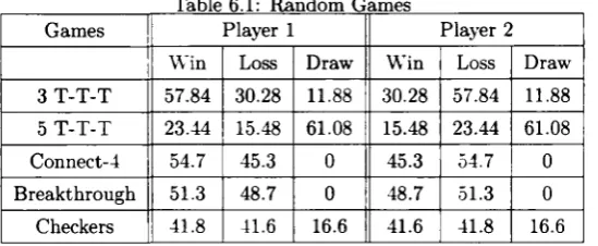
6.1 Random Games

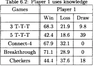
6.2 Player 1 uses knowledge

6.3 Player 2 uses knowledge

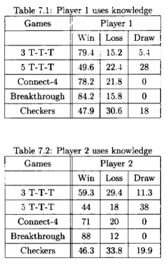
7.1 Player 1 uses knowledge

7.2 Player 2 uses knowledge

8.1 Player 1 uses coevolutionary knowledge .

8.2 Player 2 uses coevolutionary knowledge

9.1 Player 1 uses cultural and coevolutionary knowledge .

9.2 Player 2 uses cultural and coevolutionary knowledge

(12)

List of F i g u r e s

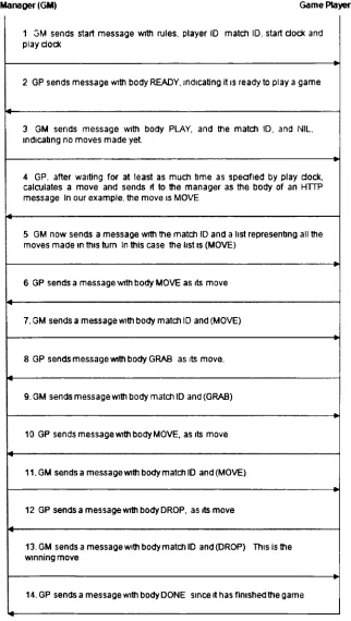
2.1 Communication between the Game Manager (GM) and the Game Player (GP) for

the game of Blocks. 12

5.1 The architecture for a general game player for learning. 26

5.2 Features in a state of Tic-Tac-Toe. The vector 9 represents the vector of features. 27

5.3 An example of knowledge representation and use while making a move in Tic-Tac-Toe. 28

6.1 The graph of the sigmoid function. 32

6.2 Temporal segmentation of features. Circular nodes are nodes from which the player

makes moves. Square nodes are the states that occur as a result of these moves (the

afterstates). 33

8.1 The forage of Antx through the Tic-Tac-Toe landscape. The presence of Anto besides

the hollow arrows indicates that Antx has the option of asking Anto for a move,

though it is not necessary to do so. Pheromone is deposited along the squiggly arrow

once a series of forages has been completed. 40

8.2 The Ant Colony G G P Architecture. 40

(13)

Chapter 1 Introduction

This thesis addresses the challenge of building intelligent General Game Playing agents. The field

of General Game Playing (GGP) is relatively new in the field of Artificial Intelligence (AI) research,

and provides an important leap in the direction and approach of the construction of intelligent agent

systems. In the past, much of the emphasis in the creation of intelligent systems was on their ability

to be proficient only for tasks they were constructed to perform. As an example, the IBM Deep Blue

computer had been constructed specifically for being good and intelligent at playing chess. However,

if any other game was given to it, it would be unable to play it as a result of its specialisation. G G P

systems, as the name implies, are far more general. They are able to accept descriptions of any

game, and are able to play them, either by making legal random moves, or legal moves made in an

intelligent manner, depending on their construction.

The importance of this research lies in the fact that G G P systems provide a step from intelligent

systems giving an illusion of intelligence to intelligent systems that act in an intelligent manner.

This difference is clear from the distinction made above between systems like Deep Blue and G G P

systems. G G P systems demonstrate their intelligence in being able to successfully play any game,

given only the rules of the game. One must delve into the areas of machine learning, knowledge

representation and pattern recognition in order to be able to construct a proficient player.

A brief overview of previous work done in the area of G G P and details of the work being

done based on the foundations laid down by Stanford University, in context of their annual G G P

competition, is now provided.

1.1 Previous work in General Game Playing

Though pure General Game Playing capabilities have not entirely been implemented, systems have

been designed which display a general behaviour with respect to a specific class of games. One

(14)

of games were formalised by [18]. Some examples of position games include Tic-Tac-Toe, Hex. the

Shannon switching games.

A position game can be defined by three sets, P, A, B. Set P is a set of positions: with set A and

B both containing subsets of P In other words, sets A and B represent a collection of subsets of P.

with each subset representing a specific positional situation of the game. The game is played with

two players, with each player alternating in moves, which consist of choosing an element from P

The chosen element cannot be chosen again. The aim for the first player is to construct one of the

sets belonging to A. whereas the aim for the second player is to construct one of the sets belonging

to B.

Programs that are capable of accepting rules of positional games, and. with practice, learn how t o

play the game have been developed. Koffman constructed a program that is able to learn important

board configurations in a 4 x 4 x 4 Tic-Tac-Toe game. This program plays about 12 times before it

learns and is effectively able to play and start defeating opponents. A set of board configurations

are described by means of a weighted graph.

1.2 T h e Stanford University G G P Project

The annual General Game Playing Competition [15] organised by Stanford University has been

instrumental in bringing about renewed interest in GGP. The rules of the games are written in

Game Description Language (GDL) [14], which is syntactically similar to prefix KIF [16]. As a

consequence, most of the current research in G G P is based on the foundations laid down by the

Stanford Group. The tournaments are controlled by the Game Manager (GM) which relays the game

information to each Game Player (GP) and checks for legality of moves and termination of the game.

Communication between players and the GM takes place in the form of H T T P messages. A more

detailed description of the architecture and game rules can be found at [1]. Successful players have

mostly focused on automatically generating heuristics based on certain generic features identified

in the game. Cluneplayer [7] was the winner of the first GGP competition, followed by Fluxplayer

[26]. Both these players, along with UTexas Larg [4] use automatic feature extraction. Evaluation

functions are created as a combination of these features and are updated in real-time to adapt to the

game. Another approach that has been taken is in [5], where transfer of knowledge extracted from

one game to another is explored by means of a TD(A) based reinforcement learner. CADIA-Player

[6] was the first General Game Player to use a simulation based approach, using UCT [17] to search

for solutions, and was the winner of the last G G P Competition. [27] also explored a Monte-Carlo

approach in which random simulations were generated and the move with the highest win rate was

selected. To improve the nature of these simulations, patterns in the sequences were extracted and

(15)

an algorithm for automatically evolving neural networks using an evolutionary approach, for G G P

1.3 Thesis Contribution

The major contributions thesis can be enumerated as follows:

1. This work represents, what is to the best of our knowledge, the first attempt at using machine

learning techniques for G G P

2. We use cultural coevolution to learn knowledge in two player, zero-sum. perfect information

deterministic games in the total absence of any prior knowledge or information about the game.

3. We demonstrate that effectiveness of this knowledge by playing various games for which the

knowledge is learnt using our approach against a standard random player. The matches are

against a random player because the current G G P format does not support learning players.

4. We combine the knowledge with UCT search, and demonstrate that this combination improves

the performance of UCT for general games.

There is a growing interest in the academic community at starting new G G P competitions that

will allow learning players to compete. As a result, there is a great scope for future work in the area

that looks into developing architecture and description languages that will suit learning players. The

work presented in this thesis is based on the format developed at Stanford, which is not conducive

to learning players. However, the principles and algorithms presented here can be used with any

game description language that allows for a random game to be played and state descriptions to be

stored and recognised. Future work which develops languages and architetures for learning players

will further complement the ideas presented in this work.

1.4 Organisation

This dissertation is organised as follows: Chapter 2 provides an overview of the G G P framework as

laid down by Stanford University, including the Game Description Language. We use this framework

as a testbed for our work. Chapters 3 and 4 provide brief introductions to Reinforcement Learning

and the Evolutionary methods that we use in our work. Chapter 5 gives the basic structure of the

player and also describes how the knowledge is represented. Chapters 6 discusses how RL can be

used in GGP. Chapters 7 to 9 discuss using complementing the RL architecture with coevolution,

ant colonies and cultural algorithms respectively. In Chapter 10 we describe how the knowledge

learnt can be used with UCT search. Finally, Chapter 11 gives the various directions for future work

(16)

C h a p t e r 2

The General Game Playing

Architecture

In this chapter, we first review a formal description of what a game is. We then look into the syntax

and semantics of the Game Description Language (GDL). The game of Tic-Tac-Toe is chosen to

provide an example on how the GDL is written and interpreted. Then, we describe the basic

communication mechanisms between the Game Manager (GM), and the Game Player (GP). We

discuss the types of messages involved in the communication, and detail out a sequence of message

exchanges between the GM and the GP for a small game. Much of the details of this chapter are

based on [14, 15].

2.1 Formal Game Description

The games considered in G G P can be considered to be finite, synchronous games. The game runs

in an environment which consists of a finite number of game states. A single state is designated

as the start state. The game also consists of one or more terminal states. The number of players

playing the game is a fixed, finite number. Whenever a player is in a game state, the player has a

finite number of actions possible from that state. All players make moves on all steps. Whether or

not they move from one state to another, or stay in the same state, is dependent on the move made,

and the state of the game at that time. The environment updates the game state only when players

make moves.

From the above description of a game, it is clear that we can view a game to be a finite state

(17)

S : A set of game states

'"li f"2, • • • • rn : The various roles, or players of an ra-player game

Ai,A2,--- ,An : Sets of actions for each player. A set At

corre-sponds to the actions possible by player rt

h- h, • • - 'n : Legal actions from a particular state. Each lt can

be considered to be a subset of Ak x S

u : An update function from one state to another

based on all the moves made

u : Ai x A2 x • • • x An x S —> S

si : The start state

Pi>92, • • • ,9n • Each gt C S x 1, • • • , 100. The value of a game

outcome for a player. For player rt, the value for

a terminal state s is given to be gt(s, value)

T : The set of terminal states. T QS

2.2 Game Description Language: GDL

A Game Description Language (GDL) is a language that can be used to describe games of complete

or partial information. It is a logical language, using logical sentences to describe rules of a game.

Syntactically, it is similar to LISP in infix notation. As we will later describe, it is relatively easy

to parse this into an equivalent form based on predicate calculus. In this section, we examine the

nature of GDL, using Tic-Tac-Toe as an example to explain it.

As a game can be viewed as a finite state machine, each game has a start state. For Tic-Tac-Toe,

the start state is a 3 x 3 gird in which each cell is blank. Therefore, we can initialise each cell to

be blank by using the init keyword of GDL in the following way (the example below illustrates only

the first row):

i n i t ( c e l l ( l , l . b ) )

i n i t ( c e l l ( l , 2 , b ) )

i n i t ( c e l l ( l , 3 , b ) )

c e l l ( x , y, z) implies that the cell in row x and column y is initialised, or set, to z. In the case

above, z is b, implying blank.

(18)

This can be done b\ the following statement:

i n i t ( c o n t r o l ( w h i t e ) )

Player one has been given the name white, and the control relation takes the players name as

the argument, and gives that player the ability to make the move.

A GDL should be able to define which moves are legal. In Tic-Tac-Toe. a move is legal for a

player if it is that players turn, and the player marks a cell that has not already been marked. In

the eventuality that neither of the conditions are true for a legal move, the player waits (the legal

action in this case is termed a noop). This can be illustrated as shown below:

legal(P.mark(M.N)) < = t r a e ( c e l l ( M . N . b ) ) k t r u e ( c o n t r o l ( P ) )

l e g a l ( v h i t e . n o o p ) < = true(cell(M.N.b)) k t r u e ( c o n t r o l ( b l a c k ) )

l e g a l ( b l a c k , n o o p ) < = t r u e ( c e l l ( M . N. b)) k t r u e ( c o n t r o l ( w h i t e ) )

In the above statements, the first statement implies that if the player P has the control (i.e.. it is

player P"s turn to move), and if the cell in row M and column N is blank, then the player is allowed to

mark that cell. Otherwise, if the control is with the other player, then the player performs a noop

action, which is an abbreviation for no operation.

Whenever a cell is marked with an X or an 0. the game states are updated. The update rules are

specified by the next predicate. These are shown as follows:

next(cell(M. N. x)) < = does(white.mark(M. N)) & t r u e ( c e l l ( M . N. b))

next(cell(M. N. o)) < = does(black,mark(M. N)) k t r u e ( c e l l ( M . N. b))

next(cell(M.N.W)) < = does(true(cell(M.N.W))) k d i s t i n c t ( W . b )

next(cell(M. N. b)) < = does(W.mark(J. K)) k t r u e ( c e l l ( M . N. V)) &

( d i s t i n c t ( M . J) | d i s t i n c t ( N . K ) )

The first two statements describe that if the control is with player white or black, then, if the cell

they are marking is blank initially, then that cell is marked with an X or an 0 respectively. The third

statement guarantees that the cell being marked is always blank. The fourth statement is an update

statement for a cell that is blank and is not marked. It ensures that if another cell, distinct from

this cell, is marked, and this cell is blank, then this cell remains blank after the move is executed.

Even- game has a set of terminal states. In Tic-Tac-Toe, these are when any single row. column

(19)

achieve these conditions, i.e., a stalemate. Therefore, the terminal states can be defined as follows:

t e r m i n a l < = l i n e ( x )

t e r m i n a l < = l i n e ( o )

t e r m i n a l < = open

While the terminal states specify the states at which if the game is, then the game is done.

However, it does not specify the goals of the players. For each player, each goal can be assigned a

numerical value. The player with the highest value of the goal wins the game. In a zero-sum game

such as Tic-Tac-Toe, there is only one winner. However, it is to be noted that not all games are

zero-sum, and games can have multiple winners. In these cases, the players with the highest goal

values win the game. In order to specify goals for Tic-Tac-Toe, we can define them as follows (only

the goals for w h i t e are shown):

g o a l ( w h i t e , 100) < = l i n e ( x )

g o a l ( w h i t e , 50) < = l i n e ( x ) & l i n e ( o ) & open

g o a l ( w h i t e , 0) < = l i n e ( o )

The goal of w h i t e is maximised when white gets a line of X's (a line in this case is either a row,

column or diagonal). The second goal specifies an example of a draw, in which neither player is able

to get a line of X's and X's. If the other player is able to get a line of 0's. then the goal value of white

becomes 0, i.e., white loses the game.

2.3 The Communication Model

The architecture of the G G P model that will be tested for this project will consist of a Game Manager

(GM) and the Game Player (GP). The Game Manager is the centralised server machine that holds

the game descriptions, allows for players to communicate and maintains the state of the overall

game. The Game Player initiates communication with the GM, during which the GM provides the

G P with the rules, written in GDL. The G P then has a limited time to learn from those rules.

Communication takes place in the form of H T T P messages that are passed between the GM and

the GP. The start message, sent to the GP by the GM, has the form of:

(START < MATCH ID > < ROLE > < GAME DESCRIPTION > < STARTCL0CK > < PLAYCLOCK > )

Where MATCH ID is the unique identification for that particular match, the ROLE is the role of

(20)

STARTCLOCK and PLAYCLOCK are integer values representing the move times. Game descriptions sent

are in the prefix form of the GDL described in the previous section.

The PLAY command takes the form:

(PLAY < MATCH ID > (< Aj > < A2 > • • • < AD > ) )

where each < An > is the action taken by the players in the previous steps. These actions are

well-ordered; the ordering sequence is specified by the game description axioms. The reply to the

PLAY command is the actual move made by the GP.

The STOP command takes the form:

(STOP < MATCH ID > (< A,. > < A2 > • • • < An >))

where each < An > is the same as what is described above in the PLAY command. This message

terminates the game.

An example of the basic communication model that is used by the General Game Playing (GGP)

server, Game manager, and the Game Player is illustrated below. The example used is that of the

game of Blocks. The valid moves for the game are MOVE, DROP and GRAB.

2.4 Implementation Details

In this chapter we will examine in detail the steps necessary for the G G P programme to take in

order to be able to successfully play a game, given the game description. The previous chapters

have examined the abstract communication model and methods to build the knowledge base from

the game rules. Now. the approach taken to facilitate the player to be able to make legal moves and

update states is described.

2.5 Updating States and Making Moves

Very briefly, the task of making a legal random move can be seen as consisting of the following steps:

1. Obtain the moves made by each player in the current turn (if the game is just starting, then

this step is ignored).

2. Use these moves to update the game states (if the game is just starting, then this step is

ignored).

3. Obtain all the legal moves that can be made in the current game state.

(21)

As we have seen from the description and syntax of the GDL, the game descriptions are written

in a logical language. Updating states and obtaining legal moves is therefore a process of inferencing

and reasoning using the rules. As we have seen in the previous chapter, converting these rules

into an equivalent Prolog code simplifies this task. This code, along with additional ground clauses

and rules, make up the knowledge base of the game. We use Prolog's inbuilt inference engine to

handle the inferencing procedures. Therefore, given all this, the task of updating states is simply

the modification of the state clauses in the knowledge base.

2.5.1 Updating the states

The states are represented as ground clauses in the knowledge base. The next predicate takes

a state description as an argument (this description represents the state valid when the moves

communicated by the GM for all players have been executed). This argument is a valid state iff

the next rule evaluates to true. If this the case, then we need to update the knowledge base by

removing the current state description, and replacing it with the argument of the next rule. In

Prolog terminology, this would imply:

1. Retract all the current state ground clauses.

2. Assert the state descriptions unified to the argument of the next rule after its evaluation.

The idea of updating states can be illustrated by a simple example. Consider the following

ground clauses and the next rule for the game of Tic-Tac-Toe:

i n i t ( c e l l ( l , l , b ) )

i n i t ( c e l l ( 1 . 2 , b ) )

i n i t ( c e l l ( 1 . 3 , b ) )

next(cell(M.N,x)) < = does(white,mark(M. N)) & true(cell(M,N.b))

If. during game play, the player with the role white marks the cell at row 1 and column 2 with an

X, then the ground clause does(white.mark(1.2,x)) is true. We need to assert this ground clause

into the knowledge base so that the next rule can be evaluated. When the Prolog inference engine

starts to evaluate the rule, the variables M and N are unified with 1 and 2 respectively. Therefore,

the new state to be asserted is c e l l ( l , 2 . x) and the state to be retracted is c e l l ( 1 . 2 , b ) .

2.5.2 Obtaining a legal move

Moves that are legal, given the current game state, are represented by the arguments to the legal

predicate in the knowledge base. Once the states are updated as described above, we need to evaluate

(22)

Now the evaluation procedure to obtain a legal move is described. The legal predicate takes two

arguments: the first argument represents the player, and the second argument represents the move

that the player can make. The constraints under which this move can be made are represented by

the predicates on the right hand side of the rule. If all these predicates evaluate to true, then the

player can make the move.

The procedure for obtaining a legal move is similar in concept to that of updating states. The

idea is to unify the variables of the rule and use the value for the move as a legal move. Prolog

automatically performs the unification during evaluation, and the legal moves can easily be collected

in a list. Therefore, t o obtain a set of legal moves, we simply call all the legal rules and collect the

assignments to the argument corresponding to the move in a list. After this, it is a simple matter

of selecting a random move and sending it to the game manager.

Below, we illustrate an example of obtaining a legal move. Consider the following clause for

making a legal move:

legal(W.mark(X.Y)) < = cell(X.Y.b) k control(W)

In the clause above, we check for two state conditions to make sure if the move represented in

the argument to legal can be made. Consider also the following state clauses:

c e l l ( l . l . b )

c e l l ( 1 . 2 . c)

c e l l ( l , 3 . b )

c o n t r o l ( w h i t e )

Assume that our role is that of white. We call the l e g a l predicate to provide us with possible

legal moves. Upon running, W is unified with w h i t e (as the current state has c o n t r o l ( w h i t e ) ) . Xow.

X and Y are first unified with 1 and 1 respectively (from the state c e l l ( l . l . b ) ) . Therefore, the first

possible legal move that we can make will be mark(l. 1). However, this is not the only move that we

can make. Notice that following the same procedure. X and Y also get unified to 1 and 3 respectively.

Therefore, another move that we can make is mark(1.3). Therefore, for the above descriptions, we

can make two legal moves. In order to make a move, we randomly select one of these moves, and

send it as a reply to the game manager as our move.

For now. we have seen how to get a list of legal moves. An important aspect of the game player

programme will be to decide which of these moves to make. In subsequent chapters, methods on

how to make intelligent legal moves will be explored. For an intelligent player, the main ideas of

(23)

(24)

Game Manager (GM) Game Player (GP)

1 3M sends start message with rules, player ID match ID, start clock and play dock

2 GP sends message with body READY, indicating it is ready to play a game

3 GM sends message with body PLAY, and the match ID, and NIL, indicating no moves made yet

4 GP. after waiting for at least as much time as specified by play dock, calculates a move and sends it to the manager as the body of an HTTP message In our example, the move is MOVE

5 GM now sends a message with the match ID and a list representing all the moves made in this turn In this case the list is (MOVE)

6 GP sends a message with body MOVE as its move

7. GM sends a message with body match ID and (MOVE)

8 GP sends message with body GRAB as its move.

9. GM sends message with body match ID and (GRAB)

10 GP sends message with body MOVE, as its move

11.GM sends a message with body match ID and (MOVE)

12 GP sends a message with body DROP, as its move

13. GM sends a message with body match ID and(DROP) This is the winning move

14. GP sends a message with body DONE since it has finished the game

(25)

Chapter 3 Reinforcement Learning

This chapter provides a brief introduction to Reinforcement Learning (RL). The G G P player relies

heavily on RL, using both Temporal Difference Learning and UCT (Upper Confidence Bounds

Applied to Trees) search. Both these topics are discussed in later sections. Much of the content of

this chapter is derived from [32] which is the standard text for RL.

Reinforcement learning is not a method or an algorithm. Its an approach, a problem solving idea.

It is different from supervised learning, where an external supervisor directs the learning by telling

the algorithm whether or not they are on the right track. What if the learning is taking place in an

unknown environment, where there just can't be a supervisor? In such a case, the agent must learn

from its experiences and interaction with the environment. This is where RL comes in.

Since RL takes place in real-time, the agent needs to constantly monitor its environment, taking

into account any unpredictable events that might happen as a result of its action, and then react

appropriately. The goals are defined explicitly for the agent, so the agent can monitor its progress

towards the goal as it takes actions and interacts with the environment, using the experience learnt

to improve its performance.

The four main features in a RL system are:

1. Policy: Given a state, what action should be taken? In other words, a policy is a mapping

from a state to a set of possible actions that can be taken from that state. It determines the

agents behaviour.

2. R e w a r d function: Indicates what is good or bad. Defines the main goal of the

reinforce-ment agent. It associates with each state or state-action pair a number, which indicates the

intrinsic desirability of that state or pair. Consequently, it provides an immediate feedback of

a situation. The aim of the agent is to maximise the total reward it receives in the long run.

(26)

3. Value function: Tells the agent the total reward it can receive from a situation. Whereas the

reward gives an immediate feedback, the value function gives the long-term feedback, taking

into account the rewards from its current situation and all possible states that are likely to

follow it.

4. E n v i r o n m e n t Model: Gives a model of the environment in which the agent is operating. It

tells the agent how the environment behaves, and what the agent can expect when it takes

actions from states.

In subsequent sections we examine the exploration-exploitation dilemma which lies at the heart

of RL, Temporal Difference Learning and Monte-Carlo Learning methods in RL.

3.1 T h e Exploration-Exploitation Dilemma

Since action selection is a core component of RL. a natural question that arises is whether an agent

should exploit actions based on what it already knows (i.e. it greedily selects the best action) or

should it instead explore new actions, with the hope of possibly increasing its reward? This is known

as the exploration-exploitation dilemma. This question also arises in the UCT algorithm described in

later chapters, where the player needs to select a move to be made and descend down the game tree.

Therefore, it is worth examining this in more detail. These questions are perhaps best explained in

the literature in the form of the N-armed bandit problem.

3.1.1 The N-Armed Bandit

The bandit in this case is an analogy to a slot machine, with N arms, and the gambler is the

agent. Each time the agent selects (or pulls) an arm, it gets a reward from a stationary probability

distribution (in other words, its not a fixed reward). A probability distribution is associated with

each arm. The goal of the agent is to maximise its total reward over a number of plays, where each

play is the selection of an arm.

Assume that for each arm, the agent maintains an estimate of its value. This value is the mean

reward it has received from that arm so far (discussed in more detail below). Now. at time step k.

what action should the agent select? The one with the highest estimate, called the greedy action

(exploitation), or a non-greedy action (exploration)? Selecting a non-greedy action may well result

in a better reward in the long run. or it may not. Deciding between exploration and exploitation

depends on many things, such as the value of the estimates, the certainty with which we know these

(27)

E s t i m a t i n g and Selecting Action-Values

The actual value of the action (i.e. play of an arm) is the mean reward received from selecting it.

However, since the distribution from which the reward comes is not known, we can only make a

guess as to what reward we will get from it. One simple way to estimate this is by keeping track

of all the rewards received for k selections for action o, and then taking the average of it. In other

words, if total plays have been t, and action a has been selected ka times, then the estimated reward

from a will be

Qt{a) = ra+r2 + rt + ... + rka ^

This is called the sample average estimate for a. As the number of plays approaches infinity.

Qt{a) will become equal to Q1 (a), which is the actual value for a.

Now that we have estimates, how do we select actions based on these estimates? A pure greedy

method would mean selecting a' for which Qt(a') = maxaQt{a). In other words, at time t, select

the action which has the highest estimated value. This would, however, mean that we never explore.

An alternative to this is selecting the greedy action most of the time, but with a small probability

e, select an action randomly, without considering its value. This is called the e — greedy action

selection method. For an infinite number of plays, each action will be sampled an infinite number

of times. If the rewards are fixed for each action, then, after selecting an action once, we know the

value. In this case, greedy action selection will work. However, most applications are non-stationary

(the rewards change over time), and so exploration is needed.

Another approach to selecting actions is by taking into account the action values. The

probabil-ities are weighted by the value of each action. So, the probability of selecting action a £ A will be

given by

eQ(«0/r

P(fl)

= E

A

W

(3

"

2)

This is called the softmax selection, r is called the temperature parameter. As r —> 0. action

selection becomes closer to greedy.

3.2 Goals and Rewards

As mentioned before, the agent attempts to maximise the long term reward (not the immediate

reward). This formalisation is a key feature in R.L; providing the agent a clear learning task.

Rewards then should be given in a clever manner, so that the agent can use them to achieve the

goal. For example, in a path finding task, if we want the agent to find the quickest route from a

(28)

a positive reward for when it reaches the ending point. Clearly, the shortest path will have the

highest reward. Another important thing to remember is that rewards are not meant to give the

agent knowledge on how to accomplish something; they are meant to tell it what to accomplish.

3.3 T h e Markov property and Markov Decision Processes

Is it necessary for the agent to know how it reached a state in order to make a decision? A good

state will tell the agent all that has happened, and at the same time retain all information that

is needed by the agent to make a decision to select an action. Such a state is said to be Markov.

In other words, all that is needed to move on to the next state is the current state, not the entire

sequence telling how you reached the current state. Formally, the Markov Property is defined as

P(st+i,<h+i\st,<h-St-i,at-i,st-2,at-2, • • • ,*o,ao) = P{st+i-at+i\st.at)

The Markov property is an important part in RL as it assumes that making decisions are a

function of only the current state.

Any RL task having the Markov property is a Markov Decision Processes (MDP), defined by the

set of states, set of actions and the one-step dynamics of the environment. A stochastic M.D.P (a

deterministic M.D.P can easily be derived from this definition) is defined as {§. A, P, E } , where S is

the set of states, A is the set of actions, P£a, gives the probability that the next state will be s' if the

agent takes action a in state s and R°s, is the expected reward rt+l the agent gets by transitioning

from state s at time step t to state s' by taking action a. Clearly, P£s, and K°3, specify the one-step

dynamics of the system.

3.4 Value functions

A value function simply tells how good a state (or a state-action pair) is. i.e. how much discounted

future reward (expected return) can be received. If a state sa gives a higher return than a state st,,

then the former has a higher value than the latter. Since a value is the expected return, which in

turn is defined by the actions that are taken from states, which in turn are defined by the policy we

follow (since a policy tells us what actions to take), values are related to specific policies.

We can define a value for a state s under a policy IT as V*(s), called the state value function, and

the value of a state-action pair (s,a) as Qn(s,a), called the action-value function. V"*(s) gives the

expected return from state s if from s we follow (select actions) policy n. Qn(s, a) gives the expected

return of taking action a from state s if, well, we take action a from state s and then follow policy

IT. Usually, a is taken using some other policy. Naturally, if a was taken using 7r itself, Qw(s, a) will

(29)

Since the values are the expected rewards starting from s or (s, a), we get

V'(a) = E^Rtlst = s} = E„ I ^rt+1+k\at = a \

Q*(s,a) = Ev{Rt\st = s.at = a} = ET I ^ rt + 1 + f c| st = s,at = a\

U=o

J

These values are represented in a tabular form, one for each state or state-action pair. Of course,

this is not the best way, as if there are too many states, then we run into a problem. Function

approximation techniques can be used t o deal with this, in which the approximators take as inputs

state parameters representing V and/or Q and output the corresponding values.

In the next section, we discuss Temporal Difference Learning. These algorithms are amongst the

most commonly used in RL problems. They do not need a model of the environment (the dynamics

of the environment) and are therefore practical for most large, real-world problems. Since we use

TD(0) for our work in this thesis, we only discuss TD(0) in the following section.

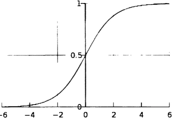
3.5 Temporal Difference Learning

Temporal Difference (TD) Learning algorithms are a family of RL algorithms that learn through

errors in the value functions at each temporal step in the state sequence. The simplest algorithm is

TD(0), which updates the value function for a state s using the error (difference) between the value

function of s, V(s), and the value function of the successor state s', V(s'). This update is shown as

V{s)i-V(s)+a[ r + -yV(s') -V(s)] (3.3)

" v ' target for TD(0)

a is called the learning rate, and usually decreases over time, r is the reward received after

tran-sitioning from s to s' The update can be thought of as moving the previous value function for s

towards the value given by the target. The update shown in Equation (3.3) is used to learn state

value functions. Algorithms such as SARSA [32] and Q-Learning [34] are used to learn action-value

functions.

Value functions are typically represented as tables, with one entry for each state or state-action

pair. However, in problems with large state spaces, this is not practical. In such cases, function

approximation techniques are used with parameterised functional forms of states, using a parameter

vector 9. State values are therefore calculated entirely from this vector, and changes are made to the

parameters instead of each individual state. The representation of the parameter vector depends on

the problem formulation.

(30)

backgam-mon player, which uses TD(A). a TD Learning algorithm. Neural Networks (NN) are used to

approximate the value functions of states, with each node in the NN corresponding to a single

pa-rameter. Using a number of simulated self-play games, TD gammon was able to reach the level of

grandmasters in backgammon.

In the next section, we describe the UCT algorithm, which uses RL to search a tree and therefore

can be used effectively for searching game trees. We also discuss how this algorithm can be used in

the G G P framework.

3.6 U C T : Upper Confidence Bound Applied to Trees

UCT [17] is an extension of the UCB1 algorithm [3], and stands for Upper Confidence Bounds

applied to Trees. The UCB1 Algorithm aims at obtaining a fair balance between exploration and

exploitation in an N-Armed bandit problem, in which the player is given the option of selecting one

of K arms of a slot machine (i.e. the bandit). This has been discussed in a previous section.

The selection of arms is directly proportional to the total number of plays and inversely

propor-tional to the number of plays of each arm. This is seen in the selection formula

The arm maximising (3.4) is selected. Xj is the average return of arm j after n plays, and Tj(n) is the

number of times it has been selected. C controls the balance between exploration and exploitation

of the tree. This formula is used in our player.

UCT extends UCB1 to trees. A single simulation consists of selecting nodes to descend down

the tree using and using (3.4) and random simulations to assign values to nodes that are being seen

for the first time. CADIA-Player [6] was the first General Game Player to use a simulation based

approach, using UCT to search for solutions, and was the winner of the last G G P Competition.

UCT has also been used in the game of Go, and the current computer world champion, Mo-Go [13].

uses UCT along with prior game knowledge. [27] also used simulations to build a basic knowledge

base of move sequence patterns in a multi-agent General Game Player. Selection of moves was done

based on the average returns, and mutation between move sequence patterns was done to facilitate

exploration. An advantage of a simulation based approach to General Game Playing is that for any

game, generating a number of random game sequences does not consume a lot of time, since no effort

is made in selecting a good move. UCT is able to guide these random playoffs and start delivering

near-optimal moves. However, even with UCT. lack of game knowledge can be a significant obstacle

in more complex games. This is because in the absence of any knowledge to guide the playoffs, it

(31)

3.6.1 UCT applied to General Games

In order to make a move the current state is set as the root node of a tree w hich is used bv L C T

To allow for adequate exploration the algorithm ensures that each child is visited at least once To

manage memory, even node that is visited at least once is added to a visited table Once a node

is reached which is not in the table a random simulation is carried on from that node till the end

of the game The reward received is backed up from t h a t node to the root Algorithm 1 shows the

basic method of UCT and the update of values in a 2 plaver zero-sum game A number of such

simulations are carried out each starting from the root and building the tree asymmetricallv

A l g o r i t h m 1 UCTSearch(root)

1 node = root

2 w h i l e visitedTable contains(node) d o 3 if node is leaf t h e n

4 r e t u r n value of node 5 else

6 if node children size == 0 t h e n 7 node createChildrenQ 8 e n d if

9 selectedChild = LCTSelect(node) 10 node = selectedChild

11 e n d if 12 e n d while

13 visitedTable add(node)

14 outcome = RandomSimulation(node) 15 while node parent / null d o 16 node visits = node visits + 1 17 node wins = node wins + outcome 18 outcome = 1 — outcome

19 node = node parent 20 e n d w h i l e

The value of each node is expressed as the ratio of the number of vv inning sequences through it

to the total number of times it has been selected In order to select the final move to be made the

algorithm returns the child of the root having the best value

3.7 Conclusions

This chapter provided a basic introduction to Reinforcement Learning (RL) It is beyond the scope

of this dissertation to provide a comprehensive overview of RL, however the reader is directed to

[32] for a more thorough mtroduction to the fundamentals of RL Indeed the material of this chapter

is adapted from this book This introduction to RL is sufficient to understand the concepts of RL

that have been used m this work

(32)

namely coevolution, ant colony optimisation and cultural algorithms.

(33)

Chapter 4 Evolutionary M e t h o d s

In this chapter we will provide a brief overview of several evolutionary methods that have been

used in our work for generating knowledge in GGP. We start by introducing coevolution and then

proceed to discuss ant colony optimisation (ACO) methods and cultural algorithms. The details of

how these are used in our work will be clearer in subsequent chapters.

4.1 Coevolution

The principle of coevolution1 can be best explained with the help of an example. Consider the

complex relationships that exist between herbivores and plants. To prevent themselves from being

eaten, plants evolve to develop defense mechanisms such as toxic leaves, thick foliage, size and thorns.

To overcome this, herbivores evolve, for example, long tongues and thick lips to overcome the foliage

and thorns and special dietary habits such as eating clay to neutralise the toxins in the leaves. Both

plants and herbivores in this case represent competing populations, each one trying to get an edge

over the other. This is the principle of coevolution; using random variation and selection to evolve

and learn strategies that will enable individuals to gain this edge that they need to survive.

A successful example of coevolution is the checkers player Blondie24 [10]. Each player is

repre-sented as a neural network which accepts as input a vector representing a checkers board position

and outputs a number in the range [—1.1] to indicate its estimation of a moves' quality. A

popu-lation of such players play against each other, alternating between roles (red or black). The top 15

individuals are selected to spawn a new generation. The best evolved network at the end of this

coevolutionary process is selected to play the game against opponents. At www.zone.com, a free

checkers game website, Blondie24 was ranked amongst the top 500 of the 120,000 registered players.

[20] and [11] also discuss the use of coevolution in evolving strategies for games such as checkers

and tic-tac-toe. The population model uses Particle Swarms. The particles are vectors of weights

(34)

of a neural network, and it is these weights that are trained using coevolution and Particle Swarm

Optimisation.

4.2 Ant Colony Optimisation Algorithms

Ant Colony Optimisation Algorithms (ACO) were developed by [8]. They take inspiration from the

behaviour of ants in nature. In nature, ants wander randomly, searching for food. Once they have

found food, they return to their colony while laying down pheromone trails These act as a guide for

other ants in the future. When other ants find such a path, instead of wandering around randomly,

they are more likely to follow the trail and further reinforce it by their pheromone deposits if they are

successful. Since pheromone evaporates over time, shorter paths are more likely to have a stronger

concentration of deposits. As a consequence, over time, short paths get favoured by more and more

ants. This approach is applied in computer science to solve optimisation and path finding problems,

such as in [9], using multiple agents (the ants) that move around in the problem space in search for

the desired solutions.

Two key parameters that determine the state transitions are the desirability (or attractiveness),

77,j, and the pheromone level, TtJ of the path (or arc) between the two states i and j . rjtj is usually

represented by a predefined heuristic, and therefore indicates an a priori fitness of the path. On the

other hand, ry indicated the past success of the move, and therefore represents a posteriori fitness

of the path. The update for T13 take place once all the ants have finished foraging. Given these two

parameters, the probability of selecting a path ptJ between states i and j is given by (4.1)

B

_ (^

a

W)

P,J

- £

Ke

„(^)(^)

(41)

a and (3 are user-defined parameters that determine how much influence should be given to the trail

strength and desirability respectively. M is the set of all legal moves that can be made from state i.

Once all the ants have finished foraging through the state space, the trails are updated as

r,_, (i) = prl3 (t - 1) + A ry (4.2)

ATV, is the cumulative accumulation of pheromone by each ant that has passed between i and j and

t represents the time step, p is called the evaporation parameter, and determines by what value

the previous trail level decreases. This gradual evaporation prevents the ants from converging to a

(35)

4.3 Cultural Algorithms

Cultural Algorithms simulate cultural evolution, bringing about a more comprehensive learning and

evolution than simple biological evolution. They can be used in both static and dynamic

environ-ments, and in complex multi-agent systems to provide effective simulations of learning procedures

[23]. Evolution takes place at both the cultural level (the belief space) and the population level

(for each individual). The belief space is the knowledge that is shared amongst the agents in the

population. This model of dual-inheritance is the key feature of Cultural Algorithms, as it allows

for a two-way system of learning and adaptation to take place. In a dual-inheritance system, the fit

population members, as selected by an acceptance function on the basis of a fitness value, add their

knowledge and experience to the belief space, thereby sharing it with all other agents in the

environ-ment. The belief space knowledge in turn helps guide the agents in the population by means of an

influence function. Other evolutionary approaches, such as Genetic Algorithms, allow for evolution

to take place only at the individual (or population) level, i.e., they do not support a dual-inheritance

system.

[24] showed that cultural learning takes place using three distinct phases of problem solving.

They defined them as coarse-grained, fine-grained and backtracking. They also discovered five types

of knowledge, namely normative (ranges of acceptable values), topographic (representing spatial

patterns), situational (successful and unsuccessful instances), historic (temporal patterns) and

do-main (relationships and interactions between dodo-main objects) knowledge. Each of the phases has a

dominance of one type of knowledge over the other.

Recent work done by [23] uses cultural algorithms to simulate the early Anasazi settlements

and answer questions regarding their disappearance from the Mesa Verde region, and is discussed

in chapter 3. This work is an example of the use of Cultural Learning in a complex multi-agent

system, in which many different factors affect the manner in which the population evolves.

To get an idea of how cultural evolution can complement coevolution, consider the following

example: assume a large herd of wilderbeests are constantly being eaten by lions. Soon, a few them

come up with a way to evade this unfortunate fate. In normal coevolution, this information would

not be shared by other members of the herd. Instead, future generations would most likely inherit

it, and so the knowledge would be passed on. However, when cultural evolution comes into play,

this knowledge of evasion is put into the herds' "belief space', and thus can be shared by other

wilderbeasts. It is the same as the clever wilderbeests going to their herd members and passing this

knowledge on to them. From a gaming perspective, players that are come up with strong strategies

are able to share them with other players, thereby allowing for faster learning and the emergence of

(36)

4.4 Conclusions

This chapter gave an overview of the evolutionary- methods that will be used in our work. Subsequent

chapters will build upon the methods introduced in this and preceding chapters and explain how

(37)

Chapter 5 Learning and Knowledge

Representation Architecture

This chapter describes the basic architecture of the multi-agent coevolutionary environment that is

used by the game player to generate game knowledge. The knowledge representation structure is

also described in detail. The terminology used in this chapter will be in context of the terminology

used in evolutionary computation. Given that in the Stanford G G P system, the lexicon of the game

rules can be changed while the underlying game logic remains the same, a way to recognise games

is also described at the end.

5.1 Player Architecture

Upon receiving the game rules, the player first calls upon the learning module to use the game

rules to learn knowledge about the game. Once the knowledge is learnt, moves are simply made by

consulting the knowledge and making the move which results in the state having the highest value

(this is explained in more detail in the next section). This is illustrated in Figure 5.1.

The learning module consists of a population of agents. Each of these agents can play the game

based on the game rules. The population is divided into a number of sub-populations, where the

number of such sub-populations is the same as the number of roles in the game. For example, Chess

has two roles, Black and White. Therefore, the number of sub-populations for Chess would be two.

These populations play against each other in a coevolutionary setup and generate knowledge for

their respective roles. The knowledge is stored and saved so that it can be used later when the game

(38)

G a m e Rules

Accept and use rules

G a m e

Player

L e a r n g a m e

I

Learning

Module

Store game

knowledge

Use knowledge

t o make moves

Figure 5.1: The architecture for a general game player for learning.

5.2 Knowledge Representation Scheme

The knowledge relates directly to the states of the game (i.e. the nodes of the game tree). The

knowledge is used to evaluate state that results from making a move, and then select the move that

gives the state with the highest value. These values are learnt using the learning module.

Since the number of states in most games is extremely large, using a table with an entry for a

value function of each state is impractical. Therefore, we approximate the state representations by

using features 1 to represent each state. In the context of the game descriptions given in GDL, this

can be done as follows. States in GDL are represented as a set of ordered tuples, each of which

specifies a certain feature of the state. For example, in Tic-Tac-Toe. mark(l, 1,X) specifies that the

cell in row 1 and column 1 is marked with an X. Therefore, a state in Tic-tac-Toe is represented as

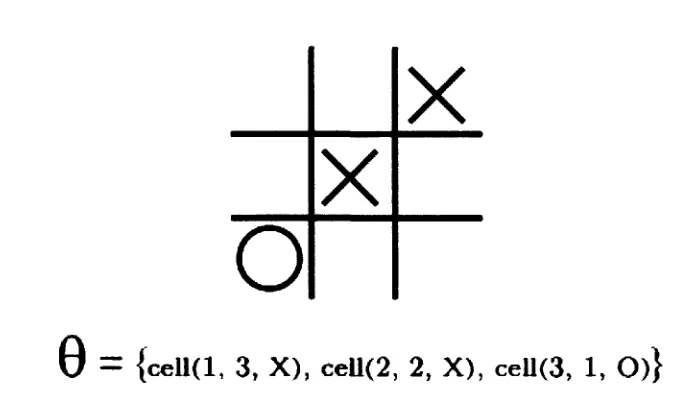
a set of 9 such tuples, each specifying whether a cell is blank or contains an X or an O. Figure 5.2

given as example of a state in Tic-Tac-Toe and the corresponding features associated with it. Xote

that the elements of the feature vector in Figure 5.2 are represented as strings for clarity. In reality,

each element 8 of the vector can be viewed as a 2-tuple (<;. v). consisting of the string <; representing

(39)

o

X

0 = {cell(l, 3, X), ceU(2, 2, X), cell(3, 1, O)}

Figure 5.2: Features in a state of Tic-Tac-Toe. The vector 9 represents the vector of features.

the feature and its corresponding value v € 9?. From now on, whenever we talk about features,

whether we are referring to the string or the value will be clear depending on the context. In GGP,

the lexicon of the game can change, but the underlying logic remains the same. Consequently, the

learning that occurs is not based on the actual strings but the values that are learnt for them.

These features are stored in a table, with entries for the various values for each feature. These

values for each feature are learnt by using the various learning algorithms that will be described in

the next chapter. To obtain the value of a state, the features present in the state are matched to the

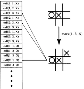
features in the tables, and their values are then used to calculate the state value. This is illustrated

in Figure 5.3. For simplicity, only a part of the table and one possible move that can be made from

the given state is shown. The actual values are omitted as they are based on the learning method

used to obtain them.

Given t h a t states are represented as shown in Figure 5.2. extracting a list of features can be done

using the simple algorithm given in Algorithm 2.

By playing a number of random games, it is possible to extract features from each state seen

after making a move and adding it to a global feature list that can be used for learning. It is possible

to do this online (during learning) or offline (prior to learning).

5.3 Recognising games independent of game rules

Since the lexicon for games written in GDL can change, it is worth looking into recognising games

based on the underlying game logic. In order to this, we use a simple technique for recognising

aspects of the game tree itself. To do this, we first play a number of random games using the given

(40)

c e l l d 1. X)

cell(l, 2 X)

cell(l 3, X)

ceU(2. 1 X)

cell(2, 2, X)

cell(2. 3 , X )

ceU(3. 1, X)

cell(3, 2, X)

ceU(3 3 , X )

c e l l d 1, O )

c e l l d 2 O )

celld 3 O )

cell(2. 1 O)

cell(2, 2 O)

mark(l, 3, X)

Figure 5 3 An example of knowledge representation and use while making a move m Tic-Tac-Toe

A l g o r i t h m 2 ExtractFeatures(startState)

initialise featureList currentState <— startState

w h i l e numberOf Games < totalGam.es d o while currentState ^ terminalState do

legalMovesList <— all legal moves possible from currentState make a legal move m £ legalMovesList randomly

observe newState reached by making m

for all feature € newState d o if feature £ featureList t h e n

add feature to featureList

end if e n d for e n d while

numberOf Games + +

1 The number of children at the given node This means keeping track of the total number of

possible legal moves that can be made from the current state in the game at each step