HPCC Benchmarking

(1)

Final Project Report

HPCC Benchmarking

MAY 29, 2018 RUSHIKESHGHATPANDE SUPERVISOR: VINCENT W FREEH

(2)

(3)

A

BSTRACT

(4)

T

ABLE OF

C

ONTENTS

Page

List of Tables iv

List of Figures v

1 Introduction 1

2 Requirements 3

2.1 Functional Requirements . . . 3

2.2 Non-Functional Requirements . . . 3

3 System Environment 5 3.1 Hardware Specifications . . . 5

3.2 Software Specifications . . . 5

4 Design, Implementation and Results 7 4.1 Design . . . 7

4.2 Implementation . . . 8

4.3 Results . . . 9

5 Observations and Challenges 13 5.1 Observation . . . 13

5.1.1 CPU Utilization . . . 13

5.1.2 Code Optimization . . . 15

5.2 Challenges . . . 15

Bibliography 17 Appendix A 19 1. Base image creation . . . 19

2. Installation of Hadoop multinode setup on Ubuntu 16.04 . . . 20

3. Installation of HPCC multinode setup on Ubuntu 16.04 . . . 20

4. HPCC Compute Kernel Code . . . 20

(5)

TABLE OF CONTENTS

5. HPCC Application Kernel Code . . . 22

6. Hadoop All Kernels Code . . . 22

(6)

L

IST OF

T

ABLES

TABLE Page

(7)

L

IST OF

F

IGURES

FIGURE Page

4.1 HPCC master . . . 9

4.2 HPCC slave 1 . . . 10

4.3 HPCC slave 2 . . . 10

4.4 M4.large computation kernels . . . 10

4.5 M4.large sort based kernels . . . 11

4.6 T2.2xlarge kernels . . . 11

4.7 Vertical scaling . . . 12

5.1 M4 CPU utilization . . . 13

5.2 Sorting CPU utilization . . . 14

(8)

(9)

C

H A P T E R

1

I

NTRODUCTION

A

s data volumes grow exponentially, the demand for flexible data analysis platforms is also growing increasingly. Data Analytics has use-cases spread across myriad of industry

domains viz., Health Care, Insurance Services, Financial Services, Character Recognition

etc. The problems of volume, velocity, and variety in the big data pervasive today has lead to many

different innovative technologies to enable its processing and extract meaningful information.

Hadoop and Spark have emerged as two of the most popular big data analytics engines. The

extensive benchmarking data, available community support and related tools have made them

popular. High-performance computing cluster (HPCC) developed by Lexis Nexis risk solutions is

also a open source platform for processing and analyzing large volumes of data.

There have been several papers discussing the performance of Hadoop and Spark. However,

not much work has been carried out in the benchmarking of HPCC platform. Tim Humphrey

et al,[2] have compared HPCC vs Spark. However, their work only involves single function

micro-level tests.

In this paper, we have evaluated the performance of HPCC Thor and Apache Hadoop for

batch processing jobs on big data. We have datasets ranging from 10 GB to 50 GB in size for

different performance tests. These performance tests can be divided into single function

micro-level tests (compute kernels) and more complex macro-micro-level tests (application kernels). HPCC

and Hadoop performance has been evaluated on parameters like scalability, time of execution

(10)

(11)

C

H A P T E R

2

R

EQUIREMENTS

T

his section elaborates the various functional and non-functional requirements that are identified as a part of our project[1]. In Section 5, each requirement is validated with a

test case and we detail the one-to-one mapping between tasks done, test case validated

and requirements satisfied.

2.1 Functional Requirements

The project ensured below mentioned functional requirements:

1. Built on Amazon Web Services

Both, Hadoop and HPCC clusters were setup on Amazon Web Services (AWS) instances.

2. Development of Test-suite

The ECL and Hadoop MapReduce codes were either self-coded or compiled from source

code. No binaries were used.

3. System-level metrics

Shell scripts were written to gather low-level metrics in a distributed AWS environment.

2.2 Non-Functional Requirements

The project ensured the below mentioned non-functional requirements:

1. Analytics platform deployed on Linux Ubuntu 16.04

The analytics platform must be deployed on Linux Ubuntu 16.04 image (detailed

(12)

CHAPTER 2. REQUIREMENTS

2. Reproducibility

The testsuite should be easily ran and evaluated on different VCL and AWS environments.

3. Extensibility

The analytics platform must allow end-user the ability to customize the test-cases and

support addition of new tests catering to his needs.

4. Testability

The developed testsuite must be easy to test and validate.

5. Installation of dependencies

All software package dependencies like Java 1.8, Python libraries etc must be installed.

(13)

C

H

A

P

T

E

R

3

S

YSTEM

E

NVIRONMENT

T

his section elaborates the specifications of our environment. Below is the list of hardware and software specifications for our project:

3.1 Hardware Specifications

The analytics platform can be deployed on bare-metal linux machines and virtual machines.

Having 4 to 8 cores will lead to a greater degree of parallelism.

The CPU architecture is Intel x86-64 and has caches of varying sizes. Each core has a 32 KB

L1 instruction and data cache, and 256 KB L2 cache. L3 cache of size 12 MB is shared among all

CPUs. The instances have had 2 to 8 cores, RAM from 4 GB to 16 GB and combined storage of

over 240 GB.

3.2 Software Specifications

Below are the software specifications for our project:

• Linux Ubuntu-16.04 LTS (Xenial Xerus) image[3] as base image.

• Apache Hadoop 2.7.5 or latest stable version.

(14)

(15)

C

H A P T E R

4

D

ESIGN

, I

MPLEMENTATION AND

R

ESULTS

I

n this section, we go into low-level details about our design decisions and their pros and cons. We further explain the implementation details of our design and the end results.

Finally, we discuss the limitations of our approach.

4.1 Design

This section describes our design decisions. The project work was divided into three main

categories. First, setting up the clusters in various environments and fine-tuning the cluster

parameters. Second, development of a test suite in Hadoop and HPCC along with the data

collection scripts. Lastly, carrying out extensive and multiple rounds of test on different cluster

types, sizes, and cloud providers.

1. Test Suite

The benchmarking test suite was divided into two categories - micro tests and macro

tests. Micro tests or ’Computational Kernels’ were single function tests for some of the

extensively used functions in big data processing like ’count’ or ’aggregate’. Macro tests or

’Application Kernels’ were the more complex tests designed which were a combination of

several functions. A low-level metrics collection script was also designed. The running of a

test suite and metrics collection script together was fully automated.

2. Dataset

The computational kernel tests were carried out on integer dataset and string datasets.

Both datasets contained several key-value based tuples. The string dataset is roughly

(16)

CHAPTER 4. DESIGN, IMPLEMENTATION AND RESULTS

consisted of 800 million records. These datasets were generated through ECL scripts shared

in the appendix section.

For application kernel tests, the data was imported from PUMA benchmark dataset. 30 GB

of histogram-based dataset was sprayed evenly across every node.

3. Cluster setup

NC State’s Virtual Cloud Laboratory (VCL) was used as a development environment for

cluster setup and building of test suite. Amazon Web Services (AWS) was used as the

production environment for gathering results.

The benchmarking experiments were carried out on AWS instances. Initially, all

experi-ments were carried out on m4.large instances in us-west-2 (Oregon) region. These instances

had 2 cores, 8 GB memory, and 200 GB EBS storage. Through our initial run, the CPU

utilization was constantly reaching a 100% and memory utilization was also severely high.

To improve the experimental setup and have a higher degree of parallelism, we decided to

vertically scale the instances. All later test runs were carried out on t2.2xlarge instances.

These instances had 8 cores and 32 GB memory. Drastic improvements and some peculiar

differences were seen for both, Hadoop and HPCC environments. EBS storage was

sup-ported by these instance types. EBS general purpose SSD volumes amounting to 200 GB

were used.

For both, Hadoop and HPCC, a 3 node cluster comprising a master node and another slave

node.

4.2 Implementation

This section describes the implementation steps for the design as explained in Section 4.1. We

explain the exact configuration steps for certain processes in the Appendix.

1. Base image setup

In the development phase, we use VCL’s imaging reservation capability to avoid

reproduc-ing a few steps related to preliminary installation. We set up our base image - Ubuntu

16.04.02 LTS (Xenial Xerus) cluster image. This image gave us capability of making cluster

reservations of any number of nodes. For further details on the exact steps involved in

installation, refer Appendix Section A.3.

2. Customized image setup with software stack installation

The next step was to create two customized images - one with HPCC 6.4.10 installed and

another with Hadoop 2.7.5 through installation of specified software packages. For further

details on the exact steps involved in installation, refer Appendix Section A.4.

(17)

4.3. RESULTS

Figure 4.1: HPCC master

3. Network , firewalls and ssh configuration

Once we set up our customized images, we ensured that there were no firewall rules

blocking any message exchange between nodes.

4. Computational Kernel Development

HPCC Computation Kernels were obtained through previous work carried out by Tim

Humphrey et al.[2]. Similar functionality was implemented for Hadoop by writing map

reduce based computational kernels in Java.

5. Application Kernel Development

Hadoop Application Kernels were obtained through PUMA Benchmark based source code[?

]. Similar functionality was implemented from scratch in ECL for HPCC environment.

6. System Metrics Script Development

A shell script with the use of ’dstat’ a Linux system monitoring tool has been implemented

to work in a distributed environment.

4.3 Results

The design and implementation details of our analytics cloud platform were explained in Sections

4.1 and 4.2. The following are the actual results of each step involved in the process of providing

the deliverables of our project.

1. Cluster deployed

Multinode HPCC and Hadoop setup were successfully installed and clusters were deployed

successfully as shown in figures 4.1-3.

2. Computational Kernel Benchmarking Results

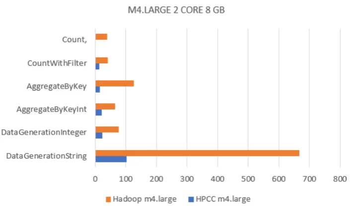
Figures 4.4 and 4.5 present the bar charts comparing the execution of several computation

kernels on m4.large cluster environments of Apache Hadoop and HPCC Thor. The first

graph contains most of the computational kernel figures while the second graph contains

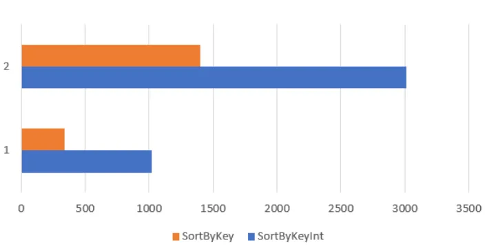
the time for sorting operation as the order of magnitude was much greater for them. It

(18)

Figure 4.2: HPCC slave 1

Figure 4.3: HPCC slave 2

Figure 4.4: M4.large computation kernels

kernel on t2.xlarge instance cluster setup. The execution times in the bar charts of figures

4.4, 4.5, and 4.6 are average execution times (averaged over 3 executions). Blue bars are for

HPCC while orange bars are for Thor. HPCC executed computational kernels a lot faster

than Hadoop.

3. Application Kernel Benchmarking Results

Figure 4.6 also presents the execution time for application kernel - which is histogram

calculation. Histogram kernel was implemented in several different ways in HPCC. The

(19)

4.3. RESULTS

Figure 4.5: M4.large sort based kernels

(20)

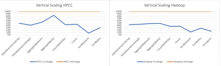
Figure 4.7: Vertical scaling

code is available in Appendix section and some observations are presented in the next

section. Hadoop performed better than HPCC for this application kernel. However,

fine-tuning of cluster and improving code quality for ECL might change that.

4. Performance VariationFigure 4.7 presents the performance of Hadoop and HPCC as we

vertically scale the instances. Hadoop’s performance greatly improved by adding more cores

and more memory. The kernels were executed on average three times faster on Hadoop after

scaling. The HPCC kernels were executed on average twice as fast on t2.xlarge machines

as m4.large. It indicates Hadoop scales better than HPCC with vertical scaling. More

information is presented in the next section.

(21)

C

H

A

P

T

E

R

5

O

BSERVATIONS AND

C

HALLENGES

V

arious experiments were carried out while consistently monitoring the system perfor-mance. Here are some interesting observations.

5.1 Observation

5.1.1 CPU Utilization

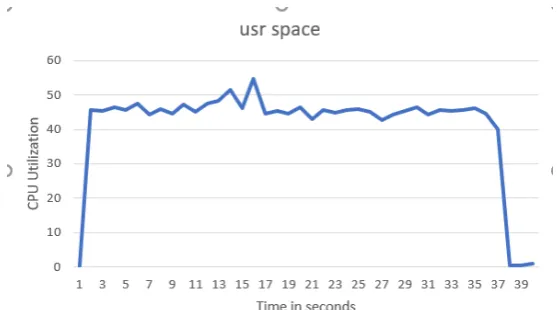
On m4.large instance, the average CPU utilization for all but one HPCC test was between 40

-50%. This percentage dropped to around 13% on HPCC t2.2xlarge instance. It may indicate that

HPCC cluster should have been setup to maximize the degree of parallelism. Hadoop scaled a lot

more linearly and no manual tuning was needed.

(22)

CHAPTER 5. OBSERVATIONS AND CHALLENGES

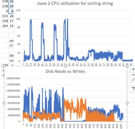
For sorting test case, however, the CPU utilization showed a peculiar wave nature as indicated

in figure 5.2. At times, the CPU utilization was at 100%. Sorting test-cases also

uncharacteris-tically took longer than expected. By superimposing the disk read / write timings on the CPU

Figure 5.2: Sorting CPU utilization

utilization time, it became clear that sorting is a disk intensive job as well. And time is spent

alternately writing to the disk and doing the actual sorting operations giving rise to the

charac-teristic pattern. In figure 5.3, in the lower half, the orange wave represents writes and the blue

wave represents reads. The upper half is again the CPU utilization pattern.

Figure 5.3: Sorting CPU utilization analysis

(23)

5.2. CHALLENGES

5.1.2 Code Optimization

HPCC compiler does several optimizations responsible for the improved performance. Some of

them are as follows:

1. The optimizer knows that the COUNT (size) is in the metadata that was created when the

dataset was created. For counting test, we don’t need to read every record instead it gets

the count from metadata.

2. For count with filter case, the optimizer creates a specialized disk count activity. Much

of the filtering is done during reading of the file, taking advantage of the latency period

between disk I/O.

3. AggregateByKeyInt kernel took same amount of time irrespective of vertically scaling the

instance.

5.2 Challenges

Several challenges were encountered in this project. They are as follows.

1. ECL language appears incredibly complex to a beginner as we are not used to declarative

programming paradigm. Hence the time for development needed for traditional developers

is a lot longer and work feels a lot harder until one gets a hang of it. It lead to us writing

fewer application kernels than what we had decided.

2. Also, it turns out, for histogram application kernel, both the codes which I wrote, although

completely distinct were not the best way to accomplish a task. All variations are added to

the appendix section.

3. The installation document for HPCC multi-node setup is not sufficient enough to make

users understand the right way to setup a cluster. HPCC has several system components

and which component to run on a particular node and how to maximize the parallelism

(24)

(25)

B

IBLIOGRAPHY

[1] AMAZONWEBSERVICES,Amazon Web Services.

https://aws.amazon.com, 2017. For using AWS.

[2] TIMOTHY L HUMPHREY , VIVEK NAIR AND JAMES MCMULLAN, Comparison of HPCC Systems_¬ÆT horvsA pacheS parkP er f ormanceonAW S.

http: // cdn. hpccsystems. com/ whitepapers/ hpccsystems_ thor_ spark. pdf, 2017.

White paper.

[3] UBUNTU,Ubuntu 16.04.2 LTS (Xenial Xerus).

http: // releases. ubuntu. com/ 16. 04/.

(26)

(27)

A

PPENDIX

A

1. Base image creation

This section of the Appendix details the steps followed to create our Ubuntu 16.04 Base image.

Following are the steps followed:

1. Download Ubuntu 16.04 ISO from ubuntu website.

2. Install qemu-kvm and virt-manager

Command –sudo apt-get install qemu-kvm; sudo apt-get install virt-manager

3. Create Qemu Image

Command –qemu-img create -f qcow2 /tmp/ubuntu_team2.qcow2 10G

4. Use virt-install to start the image installation

Command –virt-install –virt-type kvm –name ubuntu –ram 1024 cdrom=/path/to/iso/ubuntu64.iso –disk /tmp/ubuntu_team2.qcow2,format=qcow2 –network network=default -graphics vnc,listen=0.0.0.0 –noautoconsole –os-type=linux

5. Use Virt-Manager GUI to complete ubuntu installation.

6. After Completing the installation, Start the VM, Login into it and install various required

packages.

Commands –sudo apt-get install openssh-server; sudo apt-get install cloud-init cloud-utils; dpkg-reconfigure cloud-init

7. Shutdown the instance

Command –virsh stop ubuntu

8. Cleanup Mac Address

Command –virt-sysprep -d ubuntu

9. Undefine the libvirt domain

Command –virsh undefine ubuntu

10. Compress created image

(28)

APPENDIX A

11. Upload the newly created image

2. Installation of Hadoop multinode setup on Ubuntu 16.04

https://data-flair.training/blogs/hadoop-2-6-multinode-cluster-setup/ webpage provides an

excel-lent document for multinode hadoop installation.

3. Installation of HPCC multinode setup on Ubuntu 16.04

http://cdn.hpccsystems.com/releases/CE-Candidate-6.4.16/docs/Installing_and_RunningTheHPCCPlatform-6.4.16-1.pdf provides an excellent documentation for multinode HPCC installation

4. HPCC Compute Kernel Code

A.1 BWR_Ag gre gateB yK e y.ecl

WORKU N I T(0name0,0A g gre gateB yK e y0);

uniqueke ys:=100000;

unique_values:₌10212;

datasetname:=0 benchmark::strin g0;

rs:=inte gerke y,inte ger f ill;

rs_str:₌strin g10ke y,strin g90f ill;

outdata:₌D AT ASET(datasetname,rsstr,T HOR);

outdata1 :=pro ject(outdata,trans f orm(rs,sel f.f ill:=ABS((inte ger)l e f t.f ill);sel f :=l e f t));

outdata2 :₌tabl e(outdata1,ke y,sum(grou p,f ill),ke y,F EW);

OU T PU T(COU N T(outdata2));

A.2BW R_Ag gre gateB yK e yI nt.ecl

WORKU N I T(0name0,0A g gre gateB yK e yI nt0);

datasetname:=0 benchmark::inte ger0;

rs:₌inte gerke y,inte ger f ill;

outdata:₌D AT ASET(datasetname,rs,T HOR);

outdata1 :=tabl e(outdata,ke y,sum(grou p,f ill),ke y,F EW);

OU T PU T(COU N T(outdata1));

A.3BW RCount.ecl

WORKU N I T(0name0_,0_Count0_);

outdata:₌D AT ASET(dataset_name,rs,T HOR);

OU T PU T(COU N T(outdata));

(29)

4. HPCC COMPUTE KERNEL CODE

A.4BW RCountW ithF il ter.ecl

WORKU N I T(0name0,0CountW ithF il ter0);

OU T PU T(COU N T(outdata(f ill%2₌1)));

A.5BW R_DataG enerationI nte ger.ecl

WORKU N I T(0name0,0DataG enerationI nte ger0);

I MPORT ST D;

unique_ke ys:₌100000;

uniquevalues:=10212;

totalrecs:₌125000000;

unsi gned8numrecs:₌totalrecs/CLU ST ERS I ZE;

rec:=inte gerke y,inte ger f ill;

outdata:₌D AT ASET(totalrecs,trans f orm(rec,sel f.ke y:₌random()%unique_ke ys;sel f.f ill:₌

random()%uniquevalues; ),D I ST R IBU T ED);

I F(notST D.F il e.F il eExists(datasetname)

,OU T PU T(outdata, ,datasetname)

,OU T PU T(0Dataset0₊datasetname+0ALRE ADY E X I ST S.0)

);

A.6BW RDataG enerationStrin g.ecl

WORKU N I T(0name0,0DataG enerationStrin g0);

I MPORT ST D;

totalrecs:=2000000000;

unsi gned8numrecs:₌totalrecs/CLU ST ERS I ZE;

rec:=strin g10ke y,strin g90f ill;

unique_ke ys:₌100000;

uniquevalues:=10212;

ST R I NG10genke y() :=I N T FOR M AT(R AN DOM()%uniqueke ys, 10, 1);

ST R I NG10gen_fill() :₌I N T FOR M AT(R AN DOM()%unique_values, 90, 1);

outdata:₌D AT ASET(totalrecs,trans f orm(rec,sel f.ke y:₌genke y(),sel f.f ill:=genfill()),D I ST R IBU T ED);

(30)

APPENDIX A

A.7BW R_SortB yK e y.ecl

WORKU N I T(0name0,0SortB yK e y0);

sorted_dataset:₌0SortedStrin gDataS et0;

rsstr:=strin g10ke y,strin g90f ill;

outdata:₌D AT ASET(dataset_name,rs_str,T HOR);

outdata1 :₌sort(outdata,ke y);

OU T PU T(outdata1, ,sorteddataset,overwrite,CSV);

A.8BW R_SortB yK e yI nt.ecl

WORKU N I T(0name0,0SortB yK e yI nt0);

dataset_name:₌0 _benchmark_::_{inte ger}0_;

sorteddataset:=0Sorted I nte gerDataS et0;

outdata1 :₌sort(outdata,ke y);

OU T PU T(outdata1, ,sorteddataset,overwrite,CSV);

5. HPCC Application Kernel Code

ds8 := DATASET([’1:14888443, 8221095, 8850134, 308780₄,01 : 14888441, 8221095, 8850132, 308780₃],ST R I NG100l ine);

P AT T ER N d i git:=P AT T ER N(0[0−9]0);

P AT T ER N number:₌d i git₊;

P AT T ER N userRatin g:₌P AT T ER N(0₀₎

+d i git;P AT T ER N sin gl eD i git:=P AT T ER N(0_[1₋_5]0_);_{P AT T ER N l ookBe f ore}_:₌_{P AT T ER N}₍0_(?_<=₎_[1₋_5]0_);_{P AT T ER N f inalP attern}_:₌_{l ookBe f ore}₊_{l ookBe f ore}_;_{RU LEuserRatin gRul e}_:₌_{l ookBe f ore}_|_{l ookBe f ore}_;_ps_3:₌_{ST R I NG}₁₀₀_out_3:₌_{M ATCHT E X T}₍_{userRatin gRul e}_);_{ind ividualU serRatin g Answer}_:₌_{P ARSE}₍_ds_8,_{l ine}_,_{userRatin gRul e}_,_ps_3,_BEST_,_{M ANY}_,_{NOC ASE}_);_{out put}₍_{ind ividualU serRatin g Answer}_);