NOx Formation in Unsteady Counterflow Diffusion Flames

DeBruhl, Christopher Dwayne. NOx Formation in Unsteady Counterflow Diffusion

Flames. (Under the direction of Dr. William L. Roberts)

The formation of NO and NO2 are sensitive indicators of both temperature and

residence time in a combustion environment. In this work, the NOx emission index is

measured in an unsteady counterflow diffusion flame with methane, propane or ethylene,

as a function of average strain rate and amplitude and frequency an imposed sinusoidal

oscillation. These flames varied from non-sooting to high soot loading, and from low

average strain rate to near extinction. Due to the relatively long time scales associated with

NOx formation, the effect of unsteadiness on emission index is weaker than on either

temperature or soot volume fraction. Time averaged global measurements were taken

using a NO/NOx analyzer. Methane – air results are compared with unsteady calculations

By

Christopher Dwayne DeBruhl

A thesis submitted to the Graduate Faculty of North Carolina State University

in partial fulfillment of the requirements for the Degree of

Master of Science

AEROSPACE ENGINEERING

Raleigh

2003

APPROVED BY:

________________________________ ________________________________ Dr. Fred R. DeJarnette Dr. Stefan Franzen

Advisory Committee Member Advisory Committee Member

________________________________ Dr. William L. Roberts

Biography

Christopher Dwayne DeBruhl was born in Asheville, NC on January 29, 1978, and,

after a brief period of moving around Western North Carolina, grew up in Mars Hill, NC.

He lived with his parents Larry and Marsha DeBruhl and his sister Rachel DeBruhl. He

attended Madison High School, where he enjoyed playing football, wrestling, running

track, and playing lead trumpet in the wind ensemble and jazz bands. He graduated in May

1996, and enrolled at North Carolina State University. While at NCSU Dwayne earned his

BS degree in aerospace engineering, and graduated in the spring of 2000. Dwayne then

began working toward his master’s degree, in the area of combustion research. Dwayne

will begin his professional career as an aerospace engineer at Cherry Point Marine Corps

Acknowledgements

I would first like to thank my parents, Larry and Marsha, and sister, Rachel, for

their unwavering love and support throughout my life. Without their support none of this

would have been possible. They have always been there for me and I hope that I will be

able to do the same. I would also like to thank my Love and best friend, Jeanette. I could

not have made it through the last few years without her. Thank you for being you, and

being in my life. Thank you to all the friends I have made at NCSU and, especially, in the

MAE department. You’ve made my college experience unforgettable.

Thank you to Dr. William Roberts for the experience of working on this interesting

project, and for always being there to answer questions and show support. Thank you to

Dr. Tarek Echekki for the much needed support with the all of the computational work

involved in this research. I would also like to acknowledge the support of Dr. David Mann

from the Army Research Office. Partial support has for this research has been provided

Table of Contents

LIST OF FIGURES... vi

LIST OF TABLES... viii

1 INTRODUCTION... 1

1.1 NOx Formation ... 3

1.1.1 Thermal NO Mechanism... 3

1.1.2 Prompt NOx Mechanism... 5

1.1.3 Fuel Bound NOx... 8

1.1.4 NO2 Reaction Mechanism... 8

1.2 Flamelet Theory... 9

1.3 Counterflow Diffusion Flames...13

2 DESCRIPTION OF EXPERIMENTAL APPARATUS...16

2.1 Counterflow Diffusion Flame Burner...16

2.2 NOx Analyzer...19

3 NUMERICAL METHOD...21

4 STEADY COUNTERFLOW DIFFUSION FLAMES...24

5 UNSTEADY COUNTERFLOW DIFFUSION FLAME...31

5.1 Experimental Measurements for Methane CFDF’s...31

5.2 Experimental Measurements for Propane CFDF’s...34

5.3 Unsteady Computational Results for Methane CFDF’s...37

6 CONCLUSIONS...44

6.1 Steady Propane Counterflow Diffusion Flames...44

6.2 Steady Methane Counterflow Diffusion Flames...45

6.3 Unsteady Propane Counterflow Diffusion Flames...46

6.4 Unsteady Methane Counterflow Diffusion Flames...46

6.5 Future Work...48

8 APPENDICES...55

8.1 Flow Meter Settings...55

8.1.1 Global Strain Rate Conditions for Methane Counterflow Diffusion

Flames...55

8.1.2 Global Strain Rate Conditions for Propane Counterflow Diffusion

Flames...55

List of Figures

Figure 1.1 Representation of a turbulent diffusion flame illustration a diffusion flamelet.10

Figure 1.2 The S-shaped curve showing the quenching scalar dissipation rate... 13

Figure 1.3 Sketch of a stagnation point flow field in a counterflow diffusion flame... 15

Figure 2.1 Schematic of counterflow diffusion flame burner... 16

Figure 2.2 Counterflow diffusion flame burner used in experiments... 18

Figure 2.3 California Analytical Instruments Model 400 HCLD NO/NOx analyzer used in experiments...19

Figure 3.1 Comparison of speaker induced velocity oscillations and that of the opus code... 23

Figure 4.1 Uncorrected measured NO and NOx concentration versus steady strain rate. CH4 and C3H8 are plotted on the left axis while C2H4 is plotted on the right axis due to the very high soot loading associated with ethylene... 24

Figure 4.2 Counterflow diffusion flame burner with the test section shielded from room air with a window built in for flame observation... 26

Figure 4.3 Measured steady NO and NOx concentration in ppm versus steady strain rate for C3H8 and CH4... 27

Figure 4.4 NO and NOx concentration versus strain rate for the modified burner. Both numerical and experimental results for CH4 are plotted... 28

Figure 4.5 Measured NO and NOx emission index for varying steady strain rates for C3H8 and CH4... 29

Figure 4.6 NO emission index for varying steady strain rates for CH4. Experimental data is plotted the right axis and numerical results are plotted on the left axis.... 30

Figure 5.1.1 NO concentration for methane – air flame as a function of frequency and global steady strain rate for medium velocity oscillations (a) and near flow reversal oscillations (b)... 32

Figure 5.1.3 NOEmission Index for methane – air flame as a function of frequency and global steady strain rate for medium velocity oscillations (a) and near flow

reversal oscillations (b)... 34

Figure 5.1.4 NOx Emission Index for methane – air flame as a function of frequency and

global steady strain rate for medium velocity oscillations (a) and near flow reversal oscillations (b)... 34

Figure 5.2.1 NO concentrations for propane – air flame as a function of frequency and global steady strain rate for medium velocity oscillations (a) and near flow reversal oscillations (b)... 35

Figure 5.2.2 NOx concentrations for propane – air flame as a function of frequency and

global steady strain rate for medium velocity oscillations (a) and near flow reversal oscillations (b)... 36

Figure 5.2.3 NO emission index for propane – air flame as a function of frequency and global steady strain rate for medium velocity oscillations (a) and near flow

reversal oscillations (b)... 37

Figure 5.2.4 NOx emission index for propane – air flame as a function of frequency and

global steady strain rate for medium velocity oscillations (a) and near flow reversal oscillations (b)... 37

Figure 5.3.1 Phase relationship between the peak flame temperature and unsteady strain rate...39

Figure 5.3.2 Phase relationship between NO mole fraction and peak flame temperature.. 40

Figure 5.3.3 Numerical NO concentration for methane – air flame as a function of forcing frequency, amplitude and strain rate... 41

Figure 5.3.4 Computational NOx concentration as a function of frequency and amplitude for GSR 30 s-1... 41

List of Tables

1 Introduction

NOx, composed of NO, NO2, and N2O, is a pollutant formed by the combustion of

fuel in air. In the lower atmosphere nitrogen dioxide (NO2) is converted to nitric acid

(HNO3) which is a major contributor to acid rain. NOx in the lower atmosphere is

primarily produced by sources on the surface, such as automobiles and power generation

facilities. Due to the nature of terrestrial combustion many methods can be incorporated to

control NOx emissions, primarily through control of the combustion process or after-gas

treatment. Using pre-mixed flames allows for the control of the equivalence ratio, which

has a direct effect on NOx production through a reduction in the peak flame temperature.

Ozone (O3) absorbs harmful ultra violet rays, keeping the flux of UV radiation

which reaches the surface of the Earth, at a tolerable level. In the upper atmosphere nitric

oxide (NO) is very aggressive in the destruction of ozone. This is a catalytic process

because NO is regenerated, and a few molecules of NO can be responsible for the

destruction of hundreds of O3 molecules. It is difficult for NOx produced on the surface to

reach the upper atmosphere. The primary cause of NOx in the stratosphere is high altitude

aircraft such as commercial airliners. NOx produced by these aircraft is particularly

undesirable because it is inserted directly in the ozone layer.

Due to the nature of aeropropulsion, premixing the fuel and air is generally not

feasible. Therefore, these engines use turbulent diffusion flames, which operate with a

fixed equivalence ratio of unity. This means the combustion process operates at

stoichmetric conditions and cannot be adjusted, which makes controlling NOx emissions

very difficult. Because these jet engines use turbulent diffusion flames in the combustion

The study of turbulent diffusion flames is very complicated because of its

complicated multi-component flowfield, inherently unsteady nature, and the coupled

interaction between the flowfield and chemical processes. For this reason combustion

research has focused on simplifying the problem to one with simple chemistry (single step

or reduced mechanisms) or full chemistry with a simple flow field. Neither of these

approaches accurately models the chemistry in a real turbulent diffusion flame. Flamelet

theory simplifies this analysis by treating the turbulent diffusion flame as an ensemble of

strained, laminar, one-dimensional flamelets which can be described by one variable, the

mixture fraction. The flamelet model can be extended to include the non-equilibrium

effects of finite rate chemistry by introducing a new variable, the scalar dissipation rate,

which is a function of the hydrodynamics of the flowfield. Flamelet theory will be

discussed further in section 1.2.

Previous studies have shown that laminar counterflow diffusion flames under

steady rates of strain exhibit many fundamental characteristics of flamelets (Spalding,

1961; Tsuji, 1982; Seshadri & Peters, 1988; Dixon & Lewis, 1984). Conversely, only few

studies have looked at the response of counterflow diffusion flames to unsteady strain rates

(Im et al., 1995; Sung et al., 1995; Egolfopoulos & Campbell, 1996; Im et al., 1998).

Flamelet theory assumes the flamelets respond quasi-steadily to the instantaneous imposed

strain field. Recent experimental and numerical results show this is not a good assumption

for high frequency unsteadiness (Egolfopoulos, 2000; Welle et al., 2002).

This research involved experiments designed to study a flamelet’s response to

unsteady strain rates by taking time averaged measurements of the NOx produced in a

analyzer. The flames studied vary from non-sooting to high soot loading, and from low

average strain rate to near extinction. NO and NOx measurements for both steady and

unsteady flames are compared with calculations using a modified OPPDIF code, OPUS,

included in the Chemkin package.

1.1 NO

Formation

Many researchers have studied NOx formation under many different conditions

(Hayhurst & Vince, 1983; Miller & Bowman, 1989; Bowman, 1992). Many experimental

studies have been done in premixed flames (Fenimore, 1971; Glarborg et al., 1986; Dupont

& Williams, 1998; Charlston-Goch, 2001; Konnov et al., 2003) and in coflow and jet

diffusion flames (Turns & Myhr, 1991; Turns, 1995; Smyth, 1996; Yamashita et al. 1997;

Sanders et al., 1997; Caldeira-Pires et al., 2000; Frank et al., 2000; Beltarme et al., 2001;

Dally et al., 2003). There have also been many studies in steady laminar counterflow

diffusion flames which have yielded both experimental and computational data (Hahn &

Wendt, 1981; Drake & Blint, 1989; Bonturi et al., 1996; Ravikrishna & Laurendeau, 1999;

Lee et al., 2001; Fuse et al., 2002). Few researchers have focused on NOx formation in

unsteady flowfields. In general four production pathways are for NOx are distinguishable.

These include the thermal mechanism, prompt mechanism, NO production from fuel

nitrogen, and the nitrogen dioxide mechanism.

1.1.1 Thermal NO mechanism

The thermal NO mechanism (or Zel’dovich mechanism) is comprised of the

N O NO N k + + →  ← 1 2

2 (1.1)

N O k NO O

k + + →  ← 3 4

2 (1.2)

N OH k NO H

k +

+ →  ←

5

6 (1.3)

M O M O k k + + →  ← 2 7 8

2 (1.4)

If the steady state assumption is applied to N atoms, and the concentration of NO is

assumed to be small compared to the other concentrations, and if destructive reactions are

neglected compared to the formation reactions, it can be shown that,

] ][ [ 2 ] [ 2 1 O N

k dt

NO

d ₌

(1.5)

Applying the partial equilibrium assumption to reaction 1.4 the O atom concentration can

be written as,

12 12 12

2] ( ) ( ) [

]

[O = O eqkp T RuT − (1.6)

Combining these two assumptions yields,

_dt kkp T RuT O eq N eq

NO d ] [ ] [ ) ( ) ( 2 ] [ 2 2 1 2 2 1 2 1 1 −

= (1.7)

This equation shows the strong temperature dependence, because the ki’s are exponential in

temperature, and somewhat weaker dependence on the O2 concentration of the burned gas

[O2]eq, on the NO formation rate.

Reactions 1.1-1.4 involve the O and OH radicals, which also play an important role

in the oxidation of the fuel. Therefore, it is generally necessary to couple the thermal NO

reactions with that of the fuel oxidation process. However, since the overall formation of

Zel’dovich (Zel’dovich, 1946), that the thermal NO formation reactions can be decoupled

from the fuel oxidation mechanism. Zel’dovich also said that the NO formation rates

could be calculated assuming equilibrium values of temperature and concentrations of O2,

N2, O, and OH. This is, therefore, known as the Zel’dovich mechanism (cf. Miller &

Bowman, 1989).

1.1.2 Prompt NOx mechanism

Prompt NOx is NO that is formed at a rate faster than that calculated from the

simple equilibrium thermal NOx description (Zel’dovich mechanism). The formation of

prompt NOx is not fully understood. In general three sources of prompt NOx can be

distinguished; super equilibrium, Fenimore, and nitrous oxide mechanism.

Prompt NOx can be a result of super equilibrium concentrations of O and OH in the

reaction zone. This phenomenon can accelerate the rate of the Zel’dovich mechanism.

This is because the Zel’dovich mechanism assumed that the reactions O →O  ←

2

2

1 _and

O OH O

H+ → +

 ←

2 are in partial equilibrium. Super equilibrium is most important in

diffusion flames, stirred reactors at lean conditions, and low pressure premixed flames. It

can account for as much as 80% of the NO formation in these flames (Drake & Blint,

1991).

The Fenimore prompt mechanism deals with the formation of NO in hydrocarbon

flames by a reaction sequence that is initiated by hydrocarbon radicals, which attack

nitrogen molecules. This leads to the formation of atomic nitrogen, cyanides and amines,

suggested to be responsible for the prompt NO in hydrocarbon flames such as CH, CH2,

C2, C2H, and C (Miller & Bowman, 1989), however, the major contributors have been

found to be CH, CH2, and CN radicals. The mechanism is controlled by the following

reactions,

N HCN N

CH + → +

 ← 2 H NO OH

N+ → +



← (1.8)

O NO O

N + → +

 ← 2 NH HCN N

CH + → +

 ← 2 2 2 H N H

NH + → +



← (1.9)

H NO OH

N+ → +

 ←

O NO O

N + → +

 ← 2 O OCN O

CN+ → +

 ←

2 (1.10)

NO CO O

ONN+ → +

 ←

H HCN H

CN + → +

 ← 2 OH HCN O H

CN+ → +

 ← 2 2 H N H

NH + → +



← (1.11)

O NO O

N + → +

 ← 2 H NO OH

N+ → +

 ←

Reactions 1.8 was first suggested by Fenimore (Fenimore, 1971), hence the name

Fenimore prompt mechanism. This is the most dominate step in then Fenimore

mechanism. The Fenimore mechanism dominates in fuel rich premixed flames and is also

The third prompt mechanism is the nitrous oxide mechanism. This mechanism

concerns the reactions between N2O and O. The nitrous oxide pathway is given below by

reactions 1.12-1.19. The mechanism is initiated by the reverse reaction of 1.12, at which

time the N2O formed is oxidized to NO primarily by reaction 1.13. However, NO can also

be formed by reactions 1.14-1.16. The remaining N2O is then reduced by reactions 1.12

and 1.17-1.19 (Bonturi et al., 1996).

M O N M O

N + → + +



← 2

2 (1.12)

NO NO O

O

N + → +

 ←

2 (1.13)

NH NO H

O

N + → +

 ←

2 (1.14)

NCO NO

CO O

N + → +

 ←

2 (1.15)

M NO N M O

N + → + +

 ←

2 (1.16)

2 2

2O O N O

N + → +



← (1.17)

OH N

H O

N + → +



← 2

2 (1.18)

2 2

2O OH N HO

N + → +



← (1.19)

The N2O-O mechanism becomes more important in very lean flames, and low

temperatures, and is enhanced by super-equilibrium O atom concentrations. It is also very

important at high pressures because the high pressure facilitates a higher probability of a

1.1.3 Fuel Bound NOx

Another important contributor to NOx production is nitrogen that is bound

chemically to the fuel. This can be the primary source of NOx emissions from the

combustion of fossil fuels. Fuels such as ammonia (NH3) or pyridine (C5H5N) break apart

during the oxidation process and leave N-atoms free to react with O-atoms. The extent to

which the N converts to NO is a strong function of the temperature and the fuel-to-air ratio.

It is also a strong function of the fuel nitrogen content. However, it is nearly independent

of the composition of the parent fuel molecule.

Song et al. (1981), through kinetic modeling, and Chen et al. (1982), through

laboratory experiments, showed that at φ > 1 the conversion of fuel nitrogen to NO is less

prevalent than for φ ≤ 1. Some of the NO formed under this mechanism may react with

smaller hydrocarbon radicals. This facilitates the conversion of NO, formed during the

combustion process, to cyano compounds (HCN or CN). Under fuel-rich conditions these

compounds may react to form N2. This mechanism has many common features with the

Fenimore mechanism, i.e., HCN formation (Bowman 1992).

1.1.4 NO2 Reaction Mechanism

A significant source of NOx can be attributed to nitrogen dioxide, NO2. NO2 is

mainly formed by the reactions of NO with HO2, OH, O, and O2 by the following

reactions,

OH NO HO

NO+ → +



← 2

2 (1.20)

H NO OH

NO+ → +



O NO O

NO+ → +



← 2

2 (1.22)

M NO M

O

NO+ + → +



← 2 (1.23)

Because of its short lifetime in high temperature zones most NO2 formation occurs in the

low temperature regions of the flame. Here significant amounts of HO2 can be found to

react with NO formed in high temperature regions that are transported to the low

temperature regions by diffusion. Since NO2 is sensitive to the HO2 present in low

temperature regions of the flame, as shown in equation 1.20, it is also sensitive to reactions

responsible for the formation and destruction of HO2. The most important reaction for the

formation of HO2 in low temperature zones is,

M HO M

O

H + + → +



← 2

2 (1.24)

The H-atoms needed for this reaction also come from the high temperature zone by

diffusion (Miller & Bowman, 1989).

For counterflow diffusion flames the mechanisms that are most important are the

thermal mechanism, Fennimore prompt mechanism, and the Super equilibrium

mechanism.

1.2 Flamelet Theory

Turbulent diffusion flames have a very complex flame surface caused by turbulent

eddies which cause the flame to distort and wrinkle at the large scale and augment the

diffusional transport at the small scales. In order to better understand turbulent diffusion

flames flamelet theory was developed to describe the response of these complex flame

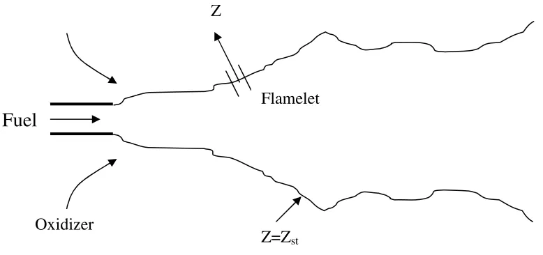
Flamelet theory treats the complex flame structure of the turbulent diffusion flame as an

ensemble of strained, laminar, one dimensional flamelets as shown in Figure 1.1.

Figure 1.1 Representation of a turbulent diffusion flame illustrating a diffusion flamelet

Burke and Schumann (1928) were the first to characterize a diffusion flame using a

conserved scalar. They suggested that the Damköhler number (Da), the ratio of fluid

dynamic time to chemical kinetic time, was infinite. The Da = ∞ assumption implies that

the flame is a one-dimensional stoichiometric surface. They also assumed single step

chemistry and a Lewis number (Le), the ratio of heat and mass diffusivities, equal to unity.

Flamelet theory says that all temperature and species profiles for the 1-D flamelet

can be completely described by a single conserved scalar for Da = ∞, Le = 1, and single

step chemistry. The conserved scalar used is the mixture fraction, Z, which is a function of

the fuel mass fraction and is bounded between zero, for pure air, and unity, for pure fuel.

0 , 0 ,

0 , O F

O

Z

β β

β β

− −

=

Fuel

Oxidizer

Z=Zst

Z

where

) (

)

( _{F F F}

F O O O O M Y M Y ν ν ν ν β _′ − ′′ − ′ − ′′ = (1.25)

YO is the mass fraction of the oxidizer, YF is the mass fraction of the fuel, M is the

molecular weight, ν′and ν′′are the stoichiometric coefficients for the reactants and

products, respectively. Using this analysis, Burke and Schumann were able to predict

flame shape and height reasonable well, for the first time. One advantage of this method is

that temperature and species profiles are linear in mixture fraction space.

In diffusion flames the mixture fraction is continuously changing throughout the

flowfield, and can be expressed as a function of the equivalence ratio. Assuming fast

chemistry, the flame is infinitely thin and exists at the stoichiometric mixture fraction

contour. The stoichiometric mixture fraction is given by,

1 2 , 1 , 1 −     ⋅ ′ ⋅ ⋅ ′ ⋅ + = F F O O O F

st _{Y M}

M Y Z ν ν (1.26)

In order to predict phenomena such as flame quenching, liftoff and blowoff, and

pollutant formation the non-equilibrium effects of finite rate chemistry must be included.

With finite rate chemistry the flame is no longer one-dimensional, but is now of finite

thickness, which is modeled as a diffusive-reactive zone. In order to account for

non-equilibrium effects an additional variable, χ, the instantaneous scalar dissipation rate, must

be introduced.

2

2D∆Z ≡

χ (1.27)

The scalar dissipation rate can be interpreted as the inverse of a characteristic

diffusion time and due to the transformation that leads to this parameter, it

incorporates the effects of convection and diffusion normal to the surface of the

stoichiometric mixture (Peters, 1984 & 1986). The scalar dissipation rate varies

inversely with Damköhler number, so as the fluid transport time gets shorter (increasing

strain rate), the dissipation rate increases. The scalar dissipation rate is a measure

of the heat conduction from both sides of the diffusive-reactive zone.

The governing equation in the region of the reactive – diffusive zone can be written

as, ) ˆ ( 2 2 2 2 ) ˆ ( ˆ _{δ ξ} γξ

ξ = y − e− y+

d y

d _(1.28)

where yˆ is the scaled mass fraction, ξ is the stretched mixture fraction variable, δ is the

reduced Damköhler number, and γ is a non-dimensional temperature. The scaled mass

fraction, stretched mixture fraction, reduced Damköhler number, and non-dimensional

temperature are given by,

γξ

− −

=( ₂)

ˆ st u a st T R E T T

y , where Ea is the activation energy (1.29)

) (Z −Zst

≡β

ξ (1.30)

3 2 ) / ( , 0

2ρ β

δ st st T R E F O Z Z D e A

Y a u st

∆

= − , where AF is the rate constant for the consumption of fuel (1.31)

      − − − − − ≡ c st o F st st

st _{T T}

T T Z ZZ

ZZ _{1 (1 )} ,0 ,0

For a given γ the governing equation can be numerically integrated to yield the maximum

temperature as a function of the reduced Damköhler number, δ. This is shown in the

S-curve in Figure 1.2. Thus if χ is increased past a critical value, χq, then the amount of heat

conducted away from the reaction zone exceeds the amount of heat generated by the

chemical reaction and the flame quenches. If equation 1.26 is evaluated at a value of Z at

the stoichiometric surface, Zst, the result is the stoichiometric scalar dissipation rate, χst.

Figure 1.2 The S-shaped curve showing the quenching scalar dissipation rate.

The two-parameter formulation assumes the flamelet responds in a quasi-steady

manner to unsteady hydrodynamics. However, recent experimental and numerical results

show that the application of unsteady strain rates to a laminar flamelet will result in a

transient response (Im et al., 1995; Welle et al., 2002).

1.3 Counterflow Diffusion Flames

Unstable solution Increasing strain rate

Da ∞

A burner comprised two opposed jets containing fuel and oxidizer impinging on a

stagnation surface is know as a counterflow diffusion flame (CFDF). A CFDF has many

essential features of a laminar diffusion flamelet and has the advantage of being very

repeatable. CFDF’ s have been used extensively to study, both experimentally and

computationally, hydrogen and light hydrocarbons flowing against air, with and without

dilution. The burner used in this study is similar to the design of Seshadri (Puri &

Seshadri, 1986), but modified to generate an unsteady flow field (Riggen-DeCroix, 1998).

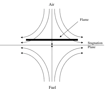
Figure 1.3 is a sketch showing a counterflow diffusion flame stabilized near the

stagnation plane of two steady, laminar opposed jets of fuel and oxidizer. For

momentum-matched opposed jets the axial velocity gradient (strain rate) is given by,

] [ , 1 2 1 5 . 0 −             + = s V V L V a o f o f o ρ ρ (1.33)

where a is the strain rate and Vo, Vf, ρf, ρo and L are the oxidizer outlet velocity, fuel outlet

velocity, fuel density, oxidizer density and burner separation distance, respectively

(Seshadri and Williams, 1978). In this study the global strain rate (GSR) is defined as

(Riggen-DeCroix, 1998),

L V

a₌2 o _(1.34)

Peters (2000) derived the scalar dissipation rate along the stoichiometric mixture

fraction contour for stagnation point flow, which is a function of the strain rate, a,

[

]

exp 2 )

( 1 2

st

st erf Z

a

Z = − ⋅ − ⋅

π

χ (1.35)

The scalar dissipation rate is a fundamental parameter as it describes the molecular mixing

important because it relates the scalar dissipation rate to an easily measured quantity, the

strain rate a.

Figure 1.3 Sketch of a stagnation point flow field in a counterflow diffusion flame

For flamelets subjected to unsteady strain rates, the scalar dissipation rate is time

dependent. Recent experimentation (DeCroix et al., 1998; Welle et al., 2000) and

computational results (Im, et al. 1995; Pitsch et al., 1998; Im, et al., 1999) has show that

these unsteady flamelets do not respond quasi-steadily as earlier expected. In fact as the

mean χ approaches the critical value, the instantaneous scalar dissipation rate may actually

exceed χq for short periods of time. The two parameter flamelet model, however, cannot

account this transient effect.

Stagnation Plane

Air

Fuel

2 Description of Experimental Apparatus

2.1 Counterflow Diffusion Flame Burner

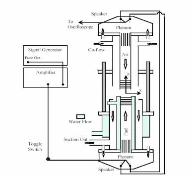
Figure 2.1 is a schematic of the counterflow diffusion flame burner used in this

experiment. The burner is similar to that described by Seshadri (Puri & Seshadri, 1986),

but has been modified to generate an unsteady flow.

The counterflow burner was operated at atmospheric pressure. The reactants flow

through 2.54 cm diameter tubes centered in the top (oxidizer side) and bottom (fuel side)

sides of the burner. The separation distance of the fuel and oxidizer tubes was held

constant at 1.27cm.

The oxidizer tube was surrounded by a 0.6 cm thick annulus for a nitrogen coflow.

This prevented preheating of the oxidizer and entrainment of ambient air into the reaction

zone. The velocity of the nitrogen coflow was set to match that of the air. The fuel tube

was surrounded by an inner water jacket to prevent preheating of the fuel. A heat

exchanger was used to cool the exhaust gases down to room temperature and prevent

preheating of the fuel. Combustion products were pumped from the test section through an

annulus by a shop-vac connected to the burner. For these experiments the suction of the

vacuum was set to 1.5 inches of water.

A 25 mesh screen was laid across the entrance of the exhaust tube to stabilize the

flame. Since the flame attached itself to the screen so there was soot deposits on the

screen. For highly sooting fuels or long running times measured NOx values began to drift

due to large deposits of soot on the screen. For this reason the screen was cleaned often.

Five one inch, 100 mesh steel screens, separated by 3mm spacers were placed in

the reactant delivery tubes. The screens flattened the exit velocity profile to be similar to a

top hat profile. Each screen was oriented at a 45° to the one above and below it. It was

found that to achieve the best results the screen at the exit of the tube needs to be a 150

mesh screen.

The unsteady flow field was imposed by using two 20cm Kicker C8a subwoofer

was set up by applying a sine wave of know frequency and amplitude to the speakers. The

sine wave was generated by a SRS Model DS335 signal generator. A McIntosh amplifier

was connected between the signal generator and the speakers to provide a 2:1 amplification

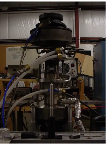
for large amplitudes. The speaker signal was monitored with an oscilloscope. A

photograph of the CFDF burner is shown in Figure 2.2.

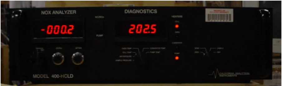
2.2 NO

Analyzer

Measurements of both NO and NOx were taken using a California Analytical

Instruments Model 400 HCLD NO/NOx analyzer (shown in Figure 2.3) as a function of

fuel type, strain rate, and amplitude/frequency of imposed oscillation. The Model 400

HCLD uses chemiluminescence to analyze the NO or NOx concentration within a gaseous

sample. It has two selectable modes NO and NOx. In the NO mode the analyzer measures

the concentration of NO in the sample and in the NOx mode it measures the concentration

of NO + NO2. A t-joint was installed down stream of the heat exchanger so the analyzer

could draw sample gases from the CFDF exhaust line.

Figure 2.3 – California Analytical Instruments Model 400 HCLD NO/NOx analyzer used in experiments.

The California Analytical Instruments Model 400 HCLD Analyzer utilizes the

principle of chemiluminescence for analyzing the NO or NOx concentration within a

gaseous sample. In the NO mode, the method is based upon the chemiluminescent reaction

Approximately 10% of the NO2 produced from this reaction is in an electronically excited

state. The transition from this excited state back down to a ground state produces a photon,

and the intensity is proportional to the number density of NO2 in the reaction chamber. The

light is measured by means of a photodiode tube and associated amplification electronics.

In the NOx mode, NO plus NO2 is determined as above, however, the sample is first routed

through the internal NO2 to NO converter which converts the NO2 in the sample to NO.

The resultant reaction is then directly proportional to the total concentration of NOx. The

3 Numerical Method

The numerical results for the steady flow field were obtained using OPPDIF (Lutz

et al., 1996). OPPDIF is a FORTRAN program that computes the diffusion flame between

two opposing nozzles. The two-dimensional axisymmetric flow field is reduced to a

one-dimensional problem using a similarity transform. Assuming that the radial component of

velocity is linear in radius, the dependent variables become functions of the axial direction

only. OPPDIF solves for the temperature, species mass fractions, axial and radial velocity

components, and radial pressure gradient, which is an eigenvalue in the problem. The

Twopnt software solves the two-point boundary value problem for the steady-state form of

the discredited equations (Lutz et al., 1996). The Chemkin packages are used to calculate

the chemical reaction rates and thermodynamic/transport properties. The chemical

mechanism used was GRI-mech 3.0 (listed in appendix 8.5) with its corresponding

thermodynamic and transport properties. Flame profiles for the species mass fraction were

spatially integrated to obtain equilibrium values for which could be compared to data

obtained from the gas analyzer. The emission index is also output by the code.

The numerical results for unsteady flow fields were computed using OPUS (Im et

al., 2000). OPUS is a FORTRAN program for computing unsteady combustion problems

in an opposed flow configuration using one-dimensional similarity coordinate. The code is

an extension of its steady counterpart, OPPDIF, to handle unsteady strain rates by

modifying the formulation to accommodate, gas dynamic compressibility effects. This

allows high-accuracy time integration with adaptive time stepping. Time integration of the

differential-algebraic system (DAE) of equations is performed by the DASPK software

for solving the DAE’ s. DASPK incorporates a variable-order, variable-step

backward-differentiation formula to solve the DAE’ s. This allows for a robust time integration of

complex unsteady problems. Like the steady code OPPDIF, OPUS also uses the Chemkin

packages to compute the associated chemical reaction rates and thermodynamic/transport

properties (Im et. al, 2000).

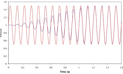
In order to accurately match the experimental velocity oscillation pattern the

function that described the unsteady velocity profile had to be rewritten. Originally the

code described the velocity as,

[

]

)

(t U AMP ft

u = _steady× + − π

However, when the function was changed to

[

]

)

(t U AMP ft

u = _steady × + π ,

the code became unstable and crashed on the first time step. After much trial and error, it

was decided that, in order to get around this problem the amplitude needed to gradually

increase to its desired value. To do this, a form of the hyperbolic tangent was incorporated

into the forcing function. After a measure of time the hyperbolic tangent would go to

unity, leaving just the sin function. Therefore, the function used was:

                + − ×

= sin(2 )

1 1 ) ( 2 1 2 2 3 3 ft e e AMP U t

u _{steady t}t π

This allowed the function to reach its desired value much faster than a normal hyperbolic

tangent function. This function is compared to a regular sine wave in Fig. 3.1. The

0 0.2 0.4 0.6 0.8 1 1.2 1.4 1.6

0 0.2 0.4 0.6 0.8 1 1.2 1.4 1.6

Time (s)

U

/U

st

ea

dy

Figure 3.1 - Comparison of speaker induced velocity oscillations and that of the opus code.

OPUS outputs species mass fractions, maximum temperature, and emission indices

as a function of time. It was also modified to output the overall species concentrations.

From this the time average values can be calculated and compared to experimental values.

4 Steady Counterflow Diffusion Flames

Readings of NO and NOx (NO + NO2) were taken for strain rates of 30, 60, 90,

120, and 150 s-1 for methane, propane, and initially ethylene. Initial measurements for

steady state methane and propane flames show that the NOx concentration increased with

strain rate as seen in Figure 4.1. This appears to run counter to what was expected so

certain steps were taken in order to validate the experimental data.

Figure 4.1 Uncorrected measured NO and NOx concentration versus steady strain rate. CH4 and C3H8 are plotted on the left axis while C2H4 is plotted on the right axis due to the very high soot loading

The first step was to express the NOx concentration in terms of the emission

index, EI. The emission index is the ratio of the mass rate of NO/NOx produced per mass

flux of fuel supplied. The emission index is give by:

4 / 2 d u m m m EI F F NO F NO

NO _{ρ π}

₌

= , [g/kg] (4.1)

where ρF is the fuel density, uF is the fuel velocity and d is the diameter of the exit tube. In

order to calculatemNOit was important to express it in terms of the mole fraction of NO,

which is easily obtained from experimentation:

products NO NO NO

NO V X V

m ₌ ρ ₌ (4.2)

From the conservation of mass it is clear that, Vproducts(slpm) is equal to the sum of

the volume flow rates of the fuel, oxidizer, and nitrogen coflow, corrected for standard

temperature and pressure, if the number of moles are equal.

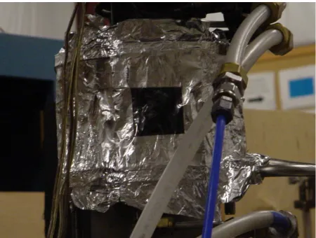
In order to accurately calculate the volume flow rates of the products it was

important to be sure that no room air was being entrained into the flame or exhaust tube

due to the low pressure annulus around the fuel tube. To do this, the burner test section

was enclosed with aluminum tape, as shown in Figure 4.2. This ensured that Vproductswas in

fact equal to VF+VO+VN2coflow.

1. Upon repeating the experiments with the enclosure, the data was seen to drastically

change from the previous results. Five runs, at each strain rate, were completed and the

error bars show that the data is very repeatable. Figure 4.3 shows the new experimental

data for C3H8 and CH4. At high steady strain rates the NO concentration, for propane,

decreases with increasing steady strain rate except between 30 and 60 s-1. Here the

concentration increases with steady strain rate, which show that more NO2 is produced at

high strain rates.

Figure 4.2 – Counterflow diffusion flame burner with the test section shielded from room air with a window built in for flame observation.

For methane, instead of increasing with strain rate, the NO concentration now

decreases with increasing strain rate as expected. The NOx concentration also decreases

with steady strain rate except between 30 and 60 Hz. This is the result that would be

expected since the flame temperature also decreases with increasing strain rate.

Experiments for C2H4 were not repeated because its high flame temperature began to melt

Figure 4.3 – Measured steady NO and NOx concentration in ppm versus steady strain rate for C3H8 and CH4.

Figure 4.4 shows the comparison between OPPDIF results and experimental data

for a methane-air flame. The experimental results matched the numerical results very well

for NO at high strain rates. However at low strain rates, particularly 30 s-1, experiment and

computation diverge. At a strain rate of 30 s-1 computational results predict twice as much

NO formation over what was experimentally measured. Even though methane is a low

sooting fuel, soot is still present at the lower strain rates, causing some of the heat to be

radiated away from the reaction zone. As the strain rate increases, the residence

time of incipient soot particles in the high temperature zone is reduced and the

a significant contribution to the total NOx production, while the numerical results show

virtually no NO2.

Figure 4.4 – NO and NOx concentration versus strain rate for the modified burner. Both numerical and experimental results for CH4 are plotted.

The emission index was also calculated and plotted for varying strain rates. Figure

4.5 shows how the emission index of NO (EINO) varies with steady strain rate for both the

experimental data for C3H8 and CH4. Here the NO emission index drops slightly with

increasing steady strain rate, while the NOx emission index remains relatively constant

Figure 4.5 - Measured NO and NOx emission index for varying steady strain rates for C3H8 and CH4.

Figure 4.6 shows how both EINO and EINOx vary with steady strain rate for

experimental and computational results for CH4. Both EINO and EINOx for the

computational data are considerably higher than their experimental counterparts. The

slope of the EINO curve from the experimental data is much steeper than that of the

predicted values. The absolute slope of the numerical curve is 7.2 x 10-3, and the

experimental is 1.83 x 10-4. This is a substantial difference. The numerical emission index

values are in good agreement with the numerical results presented by Nishioka et al.

above, while the computational emission index uses the molar production rates, similar to

that outlined by Turns (1995).

It is interesting to note contribution of NO2 to the total EINOx. As with the

concentration data the experimental EINOx has a large contribution of NO2, while the

computed values hardly has any contribution of NO2 to the total NOx.

5 Unsteady Counterflow Diffusion Flame

Measurements for the unsteady counterflow diffusion flames were also taken at

global strain rates of 30, 60, 90, 120, and 150 s-1. At each strain rate the frequency of the

loudspeakers oscillation was varied and readings were taken at 25, 50, 100, and 200 Hz for

constant amplitude. This was done for medium amplitude oscillation and an amplitude

near the flow reversal amplitude. The speaker amplitude settings are shown in Table 5.1.

Because of feedback caused by the added enclosure, previously measured applied

flow reversal voltages were no longer valid. The signal generator had to be at a much

higher voltage setting to produce the same velocity oscillation, and because of the

enclosure it was impossible to measure their exact values. This made it necessary to

visually inspect the flame to estimate the amplitude. Measurements were taken as the

flame seemed to be near the flow reversal amplitude and at roughly half the flow reversal

amplitude. This methodology was kept consistent for each strain rate.

strain rate (s-1_{) V/Vrev ~ 0.5 V/Vrev ~ 1.0 strain rate (s}-1_{) V/Vrev ~ 0.5 V/Vrev ~ 1.0}

30 1 1.5 30 1 1.5

60 1 2.5 60 1 1.5

90 2 3 90 2 3

120 2.15 3.15 120 2 3

150 2.15 3.15 150 2.15 4

Applied Speaker Voltage Applied Speaker Voltage

a) b)

Table 5.1 – Applied Speaker Voltage for a) methane – air flame and b) propane – air flame.

5.1 Experimental Measurements for Methane CFDF

Figure 5.1.1 shows the NO concentration for CH4 as a function of frequency and

global steady strain rate for medium velocity oscillations (a) and near flow reversal

concentration between 25 and 100 Hz. This drop becomes much sharper as the amplitude

reaches the flow reversal amplitude. For example, at GSR 90 s-1 the NO concentration

drops from about 1 ppm at the medium amplitude and about 3 ppm at the near flow

reversal amplitude. After the drop between 25 and 100 Hz the medium amplitude

oscillation increases roughly 1 ppm between 100 and 200 Hz. However, for the strong

velocity oscillation the NO concentration remains relatively constant between 100 and 200

Hz.

a) b)

Figure 5.1.1 - NO concentration for methane – air flame as a function of frequency and global steady strain rate for medium velocity oscillations (a) and near flow reversal oscillations (b)

Figure 5.1.2a and b show the NOx concentration for CH4-air flame as a function of

frequency and global steady strain rate. The trends for both the medium and near flow

reversal amplitudes show a drop in NOx concentration between 25 and 100 Hz. For the

medium amplitude the drop is small between 25 and 50 Hz, but between 50 Hz and 100 Hz

the drop is much steeper. This drop becomes much sharper as the amplitude reaches the

flow reversal amplitude

s-1

s-1

s-1

s-1

s-1 _ss-1

-1

s-1

s-1

After the drop between 25 and 100 Hz the medium amplitude oscillation increases

the NOx concentration roughly 1 ppm between 100 and 200 Hz. However, for the strong

velocity oscillation the NOx concentration drops about 1 ppm between 100 and 200 Hz.

The flame extinguished before reaching the near flow reversal amplitude for GSR 30 s-1

and GSR 60 s-1, which explains the increase on Figure 5.1.2b.

a) b)

Figure 5.1.2 – NOx concentration for methane – air flame as a function of frequency and global steady strain rate for medium velocity oscillations (a) and near flow reversal oscillations (b)

Figures 5.1.3 and 5.1.4 show how the NO and NOx emission index, respectively,

vary as a function of frequency, strain rate and forcing amplitude. These trends correspond

very well with the concentration data. The main notable difference is how GSR 30 s-1 is

very separated from the other strain rates. This is due to the increased nitrogen co-flow

need to stabilize the flame at the low strain rate.

s-1

s-1

s-1

s-1

s-1

s-1

s-1

s-1

s-1

a) b)

Figure 5.1.3 – NOEmission Index for methane – air flame as a function of frequency and global steady strain rate for medium velocity oscillations (a) and near flow reversal oscillations (b)

a) b)

Figure 5.1.4 – NOx Emission Index for methane – air flame as a function of frequency and global steady strain rate for medium velocity oscillations (a) and near flow reversal oscillations (b)

5.2 Experimental Measurements for Propane CFDF’s

Figure 5.2.1 shows the NO concentration for C3H8-air flame as a function of

frequency and global steady strain rate for medium velocity oscillations (a) and near flow

reversal oscillations (b). Both the medium and flow reversal amplitudes show a drop in

NO concentration between 25 and 100 Hz at strain rates of 90, 120, and 150 Hz. As with

s-1

s-1

s-1

s-1

s-1 _s-1

s-1

s-1

s-1

s-1

s-1

s-1

s-1

s-1

s-1

s-1

s-1

s-1

s-1

methane, this drop becomes much sharper as the amplitude approaches the flow reversal

amplitude. However, at strain rates of 30 and 60 Hz the NO concentration is less sensitive

to the oscillations for the medium forcing amplitude. Also, the 100 and 200 Hz

measurements for 30 and 60 Hz in Figure 5.2.1b are unreliable because the flame

extinguished before the correct amplitude could be reached.

After the drop between 25 and 100 Hz the medium amplitude oscillation increases

the concentration roughly 2 ppm between 100 and 200 Hz for the higher strain rates.

However, for the strong velocity oscillation the NO concentration only increases slightly

between 100 and 200 Hz. This is more pronounced as the strain rate increases.

a) b)

Figure 5.2.1 – NO concentrations for propane – air flame as a function of frequency and global steady strain rate for medium velocity oscillations (a) and near flow reversal oscillations (b).

Figure 5.2.2a and b show the NOx concentration for C3H8 - air flames as a function

of frequency and global steady strain rate. As with the NO concentration for propane-air

flames, the NOx concentration for both the medium and flow reversal amplitudes show a

drop in concentration between 25 and 100 Hz for global strain rates of 90 s-1 and greater.

This drop becomes more pronounced as the amplitude reaches the flow reversal amplitude.

s-1

s-1

s-1

s-1

s-1

s-1

s-1

s-1

s-1

After the drop between 25 and 100 Hz the medium amplitude oscillation increases

the NOx concentration roughly 1 ppm between 100 and 200 Hz for global strain rates of 90

and greater. However, for the strong velocity oscillation the NOx concentration drops

about 1 ppm between 100 and 200 Hz. As with the NO measurements the flame

extinguished before reaching the flow reversal amplitude for GSR 30 and GSR 60.

Figure 5.2.2 – NOx concentrations for propane – air flame as a function of frequency and global steady strain rate for medium velocity oscillations (a) and near flow reversal oscillations (b).

Figures 5.2.3 and 5.2.4 show how the NO and NOx emission index, respectively,

vary as a function of frequency, strain rate and forcing amplitude. As with the methane

emission index these trends correspond very well with the concentration data. Once again,

the main notable difference is how GSR 30 s-1 is very separated from the other strain rates.

This is due to the increased nitrogen co-flow need to stabilize the flame at the low strain

rate.

s-1

s-1

s-1

s-1

s-1

s-1

s-1

s-1

s-1

Figure 5.2.3 – NO emission index for propane – air flame as a function of frequency and global steady strain rate for medium velocity oscillations (a) and near flow reversal oscillations (b).

a) b)

Figure 5.2.4 – NOx emission index for propane – air flame as a function of frequency and global steady strain rate for medium velocity oscillations (a) and near flow reversal oscillations (b).

5.3 Unsteady Computational Results for Methane CFDF’s

Numerical calculations were done for methane – air flames subjected to unsteady

strain rates using the opus code outlined in section 3. Computations were done for strain

rates of 30, 60 and 90 s-1. At each strain rate runs of 25, 50, 100 and 200 Hz were

s-1

s-1

s-1

s-1

s-1

s-1

s-1

s-1

s-1

s-1

s-1

s-1

s-1

s-1

s-1

s-1

s-1

s-1

s-1

calculated at forcing amplitudes of one half the flow reversal amplitude, and 95% of the

flow reversal amplitude. The results were then compared to the experimental methane

data. Propane was not calculated due to the lack of a reasonably sized propane

mechanism.

Figure 5.3.1 shows how the phase of the peak flame temperature changes relative to

the calculated strain rate for increasing frequency. At 25 and 50 Hz the flame responds

quasi-steadily, because the temperature and strain rate are approximately 180 degrees out

of phase. This makes sense because, for steady laminar diffusion flames, as the strain rate

increases the temperature drops accordingly. However, as the frequency grows, the

temperature begins to move into phase with the strain rate. This is goes along with the

experimental findings of Welle (2002). Also, the NO mole fraction is directly in phase

with the temperature, as shown in Figure 5.3.2. This is to be expected because of the

nonlinear relationship between NOx formation and temperature due to the Zel’ dovich

mechanism.

b)

c)

Figure 5.3.2 – Phase relationship between NO mole fraction and peak flame temperature at frequency of 200 Hz.

Figure 5.3.3 shows the variation of NO concentration as a function of global strain

rate and frequency. The computational results show that at half of the flow reversal

amplitude the NO concentration rises slightly above the calculated steady value, and drops

slightly as the frequency increases. Between 50 and 100 Hz the concentration drops

slightly below the steady value, and remains relatively constant with further increases in

temperature. However, at 95 % of the flow reversal amplitude this effect is more

pronounced. The concentration jumps roughly 1 ppm above the steady value. As with the

medium amplitude, the high amplitude oscillation shows that the concentration drops

below the steady value between 50 and 100 Hz. It then drops even lower than the medium

amplitude, to roughly 1/3 ppm below the steady value. It is interesting to note how the

large and medium amplitudes cross the steady value at the same frequency for each global

steady computations the contribution of NO2 to the total NOx emission is very small, and

follows the same pattern as the NO concentration.

Figure 5.3.3 – Numerical NO concentration for methane – air flame as a function of forcing frequency, amplitude and strain rate.

Figure 5.3.4 – Computational NOx concentration as a function of frequency and amplitude for GSR 30 s-1_.

Steady Value

In order to better understand the experimental results it is important to directly

compare the data to calculations. Figure 5.3.5a and b shows the experimental and

computational NO concentrations for methane – air flames, plotted on the same graph for

U/Urev = 0.5 and U/Urev = 0.95 respectively. At half of the flow reversal amplitude, aside

from the already addressed difference at low strain rates, the experimental and

computational trends match up reasonably well. Both measured and calculated NO

concentration decreases as the frequency in increased up to about 100 Hz, and then

increase up to 200 Hz. However, this is much more pronounced in the experimental data,

whereas with the computational data it is much more subtle. A big difference between the

two data sets is while the experimental data shows that the imposed oscillation causes the

NO concentration to drop below the steady state value and then approach it again as the

frequency is increased, a super-equilibrium condition seems to exist with the

computational data. The imposed oscillation causes the NO concentration to rise above the

steady value, and then approach it as the frequency is increased.

At 95% of the flow reversal amplitude the experimental data still drops below the

steady value, however, the drop is much more significant. Also, after a frequency of 100

Hz the concentration no longer rises to the steady value, but rather decreases slightly. The

exact same trends can be seen in the computational data, except that the initial frequencies

a)

b)

Figure 5.3.5 - Experimental and computational NO concentrations for methane – air flames.

Steady Computational NO Value Steady Experimental NO Value

6 Conclusions

NOx emissions are a very important consideration in combustor design. Not only

are they very destructive to the natural environment, they are also hazardous to human

health and wellbeing. While NOx formation is fairly well understood in laminar diffusion

and premixed flames for simple hydrocarbons, it is not well understood for turbulent

diffusion flames or for more complex hydrocarbons. This is important because of the large

number of practical combustion devices that incorporate turbulent diffusion flames. This

research has focused on expanding the knowledge of NOx formation in steady and

unsteady counterflow diffusion flames. This research is also one of the first to

computationally and experimentally study NOx formation in unsteady counterflow

diffusion flames. The conclusions that can be drawn from this research are as follows.

6.1 Steady Propane Counterflow Diffusion Flames

2. At high steady strain rates the NO concentration, for propane, decreases with

increasing steady strain rate except at strain rates less than 60 s-1. At strain rates less

than 60 s-1 the opposite is true due to high soot loading, and thus, high radiative hear

transfer.

3. The NOx concentration increases with steady strain rate, which show that more NO2 is

produced at high strain rates. This is probably due to the fact that the high temperature

zone of the flame is narrower at high strain rates.

4. The NO emission index drops very slightly with increasing steady strain rate, while the

NOx emission index drops slightly between 30 and 60 s-1 then begins to rise with

6.2 Steady Methane Counterflow Diffusion Flames

1. The NO concentration decreases with increasing steady strain rate, as expected.

2. The NOx concentration shows a increase between 30 and 60 s-1 and then drops with

further increases in steady strain rate.

3. The NO emission index drops slightly with increasing steady strain rate, while the NOx

emission index remains relatively constant with increasing steady strain rate. The

experimental results matched the numerical results very well for NO at high strain

rates. However at low strain rates, particularly 30 s-1, experiment and computation

diverge. At a strain rate of 30 s-1 computational results predict twice as much NO

formation over what was experimentally measured. Even though methane is a low

sooting fuel, soot is still present at the lower strain rates, causing some of the heat to be

radiated away from the reaction zone. As the strain rate increases, the residence

time of incipient soot particles in the high temperature zone is reduced and

the total amount of soot decreases dramatically. According to computations

and experiments conducted by Beltrame et al. (2001), higher concentration

of soot in the flame leads to enhancement of radiant heat exchange, which

acts to reduce temperature. This could account for the reduction in the NO

concentration.

4. The OPPDIF code cannot model soot and PAH formation so the overall temperature is

predicted to be higher, corresponding to a higher NO concentration. This becomes less

predominant as the strain rate increases, because much less soot is created, hence why

5. Both EINO and EINOx for the computational data are considerably higher than their

experimental counterparts. The slope of the EINO curve from the experimental data is

much steeper than that of the predicted values. The substantial difference observed is

most probably due to the very different methods used to calculate each.

6.3 Unsteady Propane Counterflow Diffusion Flames

1. Both the medium and flow reversal amplitudes show a drop in NO concentration

between 25 and 100 Hz at strain rates of 90, 120, and 150 s-1. This drop becomes much

sharper as the amplitude reaches the flow reversal amplitude. However, at strain rates

of 30 and 60 s-1 the NO concentration is less sensitive to the oscillations for the

medium forcing amplitude.

2. Between 100 and 200 Hz the medium amplitude oscillation increases roughly 2 ppm

for the higher strain rates. However, for the strong velocity oscillation the NO

concentration only increases slightly between 100 and 200 Hz. This becomes more

pronounced as the strain rate increases.

3. The NOx concentrations follow the same trends as the NO concentration for propane –

air unsteady counterflow diffusion flames

4. The emission index also follows the same trends as the NO concentration.

6.4 Unsteady Methane Counterflow Diffusion Flames

1. Both the medium and flow reversal amplitudes show a drop in NO concentration

between 25 and 100 Hz. This drop becomes much sharper as the amplitude reaches the

oscillation increases slightly between 100 and 200 Hz. However, for the strong velocity

oscillation the NO concentration remains relatively constant between 100 and 200 Hz.

2. The trends for both the medium and flow reversal amplitudes show a drop in NOx

concentration between 25 and 100 Hz. For the medium amplitude the drop is small

between 25 and 50 Hz, but between 50 Hz and 100 Hz the drop is much steeper. This

drop becomes much sharper as the amplitude reaches the flow reversal amplitude.

After the drop between 25 and 100 Hz the medium amplitude oscillation increases the

NOx concentration slightly between 100 and 200 Hz. However, for the strong velocity

oscillation the NOx concentration drops slightly between 100 and 200 Hz.

3. The emission index trends correspond very well to the concentration data trends

4. The computations show that the temperature is initially 180 degrees out of phase with

the strain rate, but as the frequency increases the temperature begins to move into

phase with the strain rate. This matches well to previous experimental data.

5. The computed NO mole fraction is directly in phase with the temperature.

6. The experimental and computational trends match up reasonably well. Both

measurements and calculations decrease as the frequency in increased up to about 100

Hz, and then increase up to 200 Hz. However, this is much more explicit in the

experimental data, whereas with the computational data it is much more subtle. A big

difference between the two data sets is while the experimental data shows that the

imposed oscillation causes the NO concentration to drop below the steady state value

and then approach it again as the frequency is increased, a super-equilibrium condition

seems to exist with the computational data. The imposed oscillation causes the NO