A Problem With the Correlation Coefficient as a Measure of Gene Expression Divergence

(1)

DOI: 10.1534/genetics.109.110247

Note

A Problem With the Correlation Coefficient as a Measure of

Gene Expression Divergence

Vini Pereira,

1

_{David Waxman and Adam Eyre-Walker}

Centre for the Study of Evolution, School of Life Sciences, University of Sussex, Brighton BN1 9QG, United Kingdom

Manuscript received September 24, 2009 Accepted for publication September 25, 2009

ABSTRACT

The correlation coefficient is commonly used as a measure of the divergence of gene expression profiles between different species. Here we point out a potential problem with this statistic: if measurement error is large relative to the differences in expression, the correlation coefficient will tend to show high divergence for genes that have relatively uniform levels of expression across tissues or time points. We show that genes with a conserved uniform pattern of expression have significantly higher levels of expression divergence, when measured using the correlation coefficient, than other genes, in a data set from mouse, rat, and human. We also show that the Euclidean distance yields low estimates of expression divergence for genes with a conserved uniform pattern of expression.

I

T is now possible to measure the expression levels of

thousands of genes in multiple tissues at multiple times. This has led to investigations into the evolution of gene expression and how the pattern of expression changes on a genomic scale. In some analyses, the evolution of expression is considered only within one tissue, but in many studies the evolution across multiple tissues is investigated. In this latter case, the evolution of an expression profile—a vector of expression levels of a gene across several tissues—is considered.

Several different statistics have been proposed to measure the divergence between gene expression profiles. The two most popular measures are the

Euclidean distance ( Jordan et al. 2005; Kim et al.

2006; Yanai et al. 2006; Urrutia et al. 2008) and

Pearson’s correlation coefficient (Makova and Li

2003; Huminiecki and Wolfe 2004; Yanget al. 2005;

Kimet al.2006; Liao and Zhang2006a,b; Xing et al.

2007; Urrutiaet al.2008). The correlation coefficient

is often subtracted from one, so that the statistic varies from zero, when there has been no expression di-vergence, to a maximum of two; we refer to this statistic

as the Pearson distance. Here we describe a significant

shortcoming of the Pearson distance that is not shared by the Euclidean distance.

To investigate properties of these two measures of expression divergence, we compiled a data set of 2859 orthologous genes from human, mouse, and rat for which we had microarray expression data from nine homologous tissues: bone marrow, heart, kidney, large intestine, pituitary, skeletal muscle, small intestine, spleen, and thymus). The expression data for rat came

from Walkeret al.(2004), the mouse data from Suet al.

(2004), and the human data from Geet al.(2005). Each

tissue experiment had two replicates in mouse, a varying number of replicates in rat, and one in humans; some genes were also matched by multiple probe sets. To obtain an average across experiments and probe sets we processed the data as follows:

i. Raw CEL files of gene expression levels were obtained from the NCBI Gene Expression Omnibus database (http://www.ncbi.nlm.nih.gov/projects/geo/). ii. The results from the mouse, rat, and human arrays

were normalized separately using both the MAS5

(Affymetrix 2001) and the RMA algorithms

(Irizarryet al.2003) as implemented in

Bioconduc-tor (Gentlemanet al.2004). The results are

qualita-tively similar for the two normalization procedures, although recent analyses suggest that MAS5

normal-ization is generally better (Ploneret al. 2005; Lim

et al.2007).

iii. The expression of each gene within a tissue was averaged across experiments and probe sets.

Supporting information is available online athttp://www.genetics.org/

cgi/content/full/genetics.109.110247/DC1.

1_{Corresponding author:}_{Theoretical Systems Biology, Institute of Food}

Research, Norwich Research Park, Colney, Norwich NR4 7UA, United

Kingdom. E-mail: [email protected]

(2)

We computed expression distances (ED) between orthologous gene expression profiles, for each of the three species comparisons, rat–mouse, rat–human, and mouse–human, according to the two different distance metrics, the Euclidean distance and the Pearson distance:

EucD¼

ffiffiffiffiffiffiffiffiffiffiffiffiffiffiffiffiffiffiffiffiffiffiffiffiffiffiffiffiffiffi Xk

j¼1

ðx1jx2jÞ2 v

u u t

PeaD¼1

Pk

j¼1ðx1jx1Þðx2jx2Þ ffiffiffiffiffiffiffiffiffiffiffiffiffiffiffiffiffiffiffiffiffiffiffiffiffiffiffiffiffiffiffiffiffiffiffiffiffiffiffiffiffiffiffiffiffiffiffiffiffiffiffiffiffiffiffiffiffiffiffiffiffiffiffiffiffi Pk

j¼1ðx1jx1Þ2Pkj¼1ðx2jx2Þ2

q :

ð1Þ

Here xij is the expression level of the gene under

consideration in species i in tissue j, and xi is the

average expression level of the gene in speciesiacross

tissues. Expression levels are known in a total ofktissues.

Because expression levels are measured on different microarray platforms in the three species, we compute relative abundance (RA) values, before calculating the

Euclidean distance (Liaoand Zhang2006a). The RA is

the expression of a gene in a particular tissue divided by the sum of the expression values of that gene across all tissues. We calculated RA values to remove ‘‘probe’’ effects (the tendency for a gene to bind its probe set on one platform more efficiently than on another platform). Because of probe effects it is not easy to distinguish absolute changes in expression and differences in bind-ing efficiency. Calculatbind-ing RA values removes this problem from the Euclidean distance. Pearson’s distance does not change under such a rescaling and so this is unnecessary.

In some analyses the logarithm of the expression or RA

values are used (e.g., Makovaand Li2003; Kimet al.2006;

Xinget al.2007), and in others the expression values are

used without this transformation (e.g., Huminieckiand

Wolfe2004; Jordanet al.2005; Yanget al.2005; Liao

and Zhang 2006a,b; Yanai et al.2006; Urrutiaet al.

2008). We calculated both the Pearson and the Euclidean distances on log-transformed and untransformed expres-sion values. The results are qualitatively similar so here we present only the results obtained using the logarithm of the expression or RA values.

It is natural to expect the two measures of expression divergence to be positively correlated with one another; however, the Euclidean and Pearson distances are almost completely uncorrelated (MAS5 normalization,

mouse–rat correlation coefficient¼0.06, human–ratr¼

0.13, human–mouse r ¼ 0.10; RMA normalization,

mouse–rat correlation coefficient¼ 0.12, human–rat

r ¼ 0.00, human–mouser ¼ 0.08; Figure 1). This

could, plausibly, be because the two statistics measure different aspects of divergence. However, irrespective of this, there is a potential problem associated with the Pearson distance. Imagine that we have a gene that is

expressed at identicallevels in all tissues in two species

(i.e., expression levels are uniform between tissues and

Figure 1.—The correlation between the Euclidean and

Pearson distances for (a) mouse–rat, (b) human–rat, and (c) human–mouse. Only the results from MAS5 normaliza-tion are shown; qualitatively similar results were obtained with RMA.

(3)

also between species). We quite reasonably assume that measured expression levels contain noise. Thus each measured expression level (xij) is the sum of the

(as-sumed) uniform expression level and an independent random number representing noise. In this case there is no real divergence in the expression profile between the species. However, the two measures of divergence may differ greatly in this case. The Euclidean distance re-flects only the noise present in the data and hence will be small if the noise is small. By contrast, the Pearson distance will have a value close to 1 since the second term in PeaD in Equation 1 will be close to zero, reflecting the fact that the noise components of different expression levels are independent. Thus the Pearson distance will give the impression that expression divergence is great, but all this apparent divergence is noise. This will be a problem with Pearson’s distance whenever measure-ment error is of the same magnitude as the differences in expression between tissues. This will therefore tend to be a problem for lowly expressed genes, where measure-ment error can be large relative to the true value.

The above example is unrealistic because real gene expression profiles are rarely perfectly uniform. To investigate whether this shortcoming of the Pearson distance is a problem in real data sets, we determined genes with a relatively uniform pattern of expression in all three species considered above. To do this we

computed theentropyof a gene’s expression, which is a

measure of uniformity in expression across tissues (Schuget al.2005): the higher the value of the entropy, the more uniform is the expression. We calculated the entropy for each gene in each of the three species, averaged these across species, and then took those genes in the upper quartile of mean entropy values as a data set of genes with a relatively conserved pattern of uniform expression.

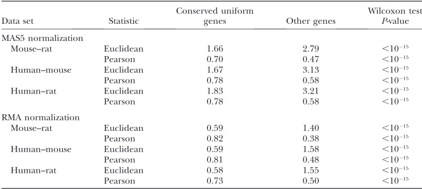
It is natural to expect those genes with a conserved uniform pattern of expression to have relatively low expression divergence; however, on average these genes have significantly higher Pearson distances than other

genes (Table 1; Figure 2; supporting information,

Figure S1 and Figure S2). By contrast, the Euclidean TABLE 1

The median expression divergence for genes that have a conserved uniform pattern of expression (upper quartile of mean entropy values)vs.all other genes

Data set Statistic

Conserved uniform

genes Other genes

Wilcoxon test

P-value

MAS5 normalization

Mouse–rat Euclidean 1.66 2.79 ,1015

Pearson 0.70 0.47 ,1015

Human–mouse Euclidean 1.67 3.13 ,1015

Pearson 0.78 0.58 ,1015

Human–rat Euclidean 1.83 3.21 ,1015

Pearson 0.78 0.58 ,1015

RMA normalization

Mouse–rat Euclidean 0.59 1.40 ,1015

Pearson 0.82 0.38 ,1015

Human–mouse Euclidean 0.59 1.58 ,1015

Pearson 0.81 0.48 ,1015

Human–rat Euclidean 0.58 1.55 ,1015

Pearson 0.73 0.50 ,1015

Figure2.—The distribution of expression di-vergence values for those genes with a uniform pattern of expression that is conserved across

species vs. the distribution for all genes for

(a) Pearson and (b) Euclidean distances

for mouse–rat. We present similar values for

human–mouse and human–rat in Figure S1

(4)

distance shows the pattern one would anticipate; all of the conserved uniform genes have low expression divergence. It therefore seems likely that the Pearson distance is sensitive to measurement error and hence may not be a good measure of expression divergence.

We note that there are two additional advantages of the Euclidean distance. First, it can take into account differences in the absolute level of expression if those data are available, either because the method of assay allows this, for example, if ESTs, SAGE, sequencing, or RNA-Seq data are used, or because expression in the two species has been assessed on the same platform using probes that are conserved between the two species. Second, the square of the Euclidean distance is

ex-pected to increase linearly with time. Khaitovichet al.

(2004) have previously shown that the squared differ-ence in log expression level increases linearly with time under a Brownian motion model of gene expression evolution. It is therefore expected that the squared Euclidean distance will increase with time since the squared Euclidean distance is the sum of the squared

differences across tissues. We prove this inFile S1; we

also show that this linearity holds, approximately, when

relative abundance values are used (see also Pereira

et al.2009).

We are grateful to a referee for helpful comments. V.P. and A.E.W. were supported by the Biotechnology and Biological Sciences Re-search Council.

LITERATURE CITED

Affymetrix_{, 2001} _{Statistical Algorithms Reference Guide.}_Affymetrix,

Santa Clara, CA.

Ge_{, X., S. Y}amamoto_{, S. T}sutsumi_{, Y. M}idorikawa_{, S. I}hara_{et al.}_,

2005 Interpreting expression profiles of cancers by genome

wide survey of breadth of expression in normal tissues. Genomics

86:127–141.

Gentleman_{, R. C., V. J. C}arey_{, D. M. B}ates_{, B. B}olstad_,

M. Dettlinget al., 2004 Bioconductor: open software

develop-ment for computational biology and bioinformatics. Genome

Biol.5:R80.

Huminiecki, L., and K. H. Wolfe, 2004 Divergence of spatial gene

expression profiles following species-specific gene duplications

in human and mouse. Genome Res.14:1870–1879.

Irizarry_{, R. A., B. H}obbs_{, F. C}ollin_{, Y. D. B}eazer_-Barclay_,

K. J. Antonelliset al., 2003 Exploration, normalization, and

summaries of high density oligonucleotide array probe level data.

Biostatistics4:249–264.

Jordan, I. K., L. Marino-Ramirez and E. V. Koonin, 2005

Evo-lutionary significance of gene expression divergence. Gene345:

119–126.

Khaitovich_{, P., G. W}eiss_{, M. L}achmann_{, I. H}ellmann_{, W. E}nard

et al., 2004 A neutral model of transcriptome evolution. PLoS

Biol.2:E132.

Kim, R. S., H. Jiand W. H. Wong, 2006 An improved distance

mea-sure between the expression profiles linking co-expression and

co-regulation in mouse. BMC Bioinformatics7:44.

Liao, B.-Y., and J. Zhang, 2006a Evolutionary conservation of

ex-pression profiles between human and mouse orthologous genes.

Mol. Biol. Evol.23:530–540.

Liao_{, B. Y., and J. Z}hang_{, 2006b} _{Low rates of expression profile}

di-vergence in highly expressed genes and tissue-specific genes

during mammalian evolution. Mol. Biol. Evol.23:1119–1128.

Lim, W. K., K. Wang, C. Lefebvre and A. Califano,

2007 Comparative analysis of microarray normalization

proce-dures: effects on reverse engineering gene networks.

Bioinfor-matics23:i282–i288.

Makova_{, K. D., and W. H. L}i_{, 2003} _{Divergence in the spatial pattern}

of gene expression between human duplicate genes. Genome

Res.13:1638–1645.

Pereira, V., D. Enardand A. Eyre-Walker, 2009 The effect of

transposable element insertions on gene expression evolution

in rodents. PLoS ONE4:e4321.

Ploner, A., L. D. Miller, P. Hall, J. Bergh and Y. Pawitan,

2005 Correlation test to assess low-level processing of

high-density oligonucleotide microarray data. BMC Bioinformatics6:80.

Schug_{, J., W. P. S}chuller_{, C. K}appen_{, J. M. S}albaum_{, M. B}ucan_{et al.}_,

2005 Promoter features related to tissue specificity as measured

by Shannon entropy. Genome Biol.6:R33.

Su, A. I., T. Wiltshire, S. Batalov, H. Lapp, K. A. Chinget al.,

2004 A gene atlas of the mouse and human protein coding

transcriptomes. Proc. Natl. Acad. Sci. USA101:6062–6067.

Urrutia_{, A. O., L. B. O}cana_{and L. D. H}urst_{, 2008} _{Do Alu repeats}

drive the evolution of the primate transcriptome? Genome Biol.

9:R25.

Walker_{, J. R., A. I. S}u_{, D. W. S}elf_{, J. B. H}ogenesch_{, H. L}app_{et al.}_,

2004 Applications of a rat multiple tissue gene expression data

set. Genome Res.14:742–749.

Xing, Y., Z. Ouyang, K. Kapur, M. P. Scott and W. H. Wong,

2007 Assessing the conservation of mammalian gene

expres-sion using high-density exon arrays. Mol. Biol. Evol.24:1283–

1285.

Yanai, I., J. O. Korbel, S. Boue, S. K. McWeeney, P. Borket al.,

2006 Similar gene expression profiles do not imply similar

tis-sue functions. Trends Genet.22:132–138.

Yang, J., A. I. Suand W. H. Li, 2005 Gene expression evolves faster

in narrowly than in broadly expressed mammalian genes. Mol.

Biol. Evol.22:2113–2118.

Communicating editor: I. Hoeschele

(5)

Supporting Information

http://www.genetics.org/cgi/content/full/genetics.109.110247/DC1

A Problem With the Correlation Coefficient as a Measure of Gene

Expression Divergence

Vini Pereira, David Waxman and Adam Eyre-Walker

Copyright © 2009 by the Genetics Society of America

(6)

V. Pereira et al.

2 SI

! "#$%&'( )+, +,' -$##'&.+$/ -$'0-*'/+ .1 . ('.12#' $3 4'/'

'5"#'11$/ 67'#4'/-'8

!"##$%&%'()+ ,'-.&)(,.'

/,', 0%%,)1 2)3,4 5)6&)' 7 84)& 9+%:5)$;%

<' (=,> >"##$%&%'()+ ,'-.&)(,.' ?% %>()@$,>= (?. %>"$(> "'4% ) *)':

4.& ?)$; &.4%$ .- A%'% %6#%>>,.' -.& )' )'B%>()$ >()(%C D,E F=% >G")%

.- (=% 9"B$,4%)' 4,>()'B% .- A%'% %6#%>>,.' #.H$%> ,'B*%)>%

!"#$%&!' (")*

)"+$

C D,,E F=% 9"B$,4%)' 4,>()'B% .- (=% *%$)(,3% )@"'4)'B% 3)$"%> .- ) A%'%

%,,&-."+%)$!'

,'B*%)>%>

!"#$%&!' (")* )"+$

C DF=% *%$)(,3% )@"'4)'B% 3)$"%

) A%'% ,' ) (,>>"% ,> ,(> %6#*%>>,.' $%3%$ ,' (=)( (,>>"% 4,3,4%4 @+ (=% >"&

.-,(> %6#%>>,.' 3)$"%> .3% )$$ (,>>"%>EC

5% B.'>,4%* %3.$"(,.' .- A%'% %6#%>>,.' $%3%$> .- ) '"&@% .- 4,I%*%'(

A%'%> ,'

!

(,>>"%>C J%(

"

!

4%'.(% (=% %6#%>>,.' $%3%$ .- ) #)(,B"$)* A%'%1

,' ) #)(,B"$) >#%B,%>1 ,' (,>>"%

#C 5% B.$$%B( (=%>% %6#*%>>,.' $%3%$> ,'(.

) 3%B(.*

!

"

!

$ "

"

$ %%%$ "

"

%#%>%'(,'A (=% %6#*%>>,.' $%3%$ .- (=% A%'% ,' )$$

!

(,>>"%> )'4 %-% (. (=,> 3%B(.* )> (=% %6#%>>,.' $%3%$ #.H$% .- (=% A%'%C

5% &);% (=% )>>"&#(,.' (=)( (=% %6#%>>,.' $%3%$> .- 4,I%%'( A%'%>1 ,'

4,I%%'( (,>>"%>1 )% (=% ."(B.&% .-

"#/$,$#/$#) +0!)",!"1%)"2$ &%#/-+ (%!34

-.& )' )'B%>()$ %6#%>>,.' $%3%$C F=% )'B%>(. ,> ();%' (. .BB"* )( (,&%

&

# $

)'4 (=% %6#%>>,.' $%3%$ .- ) #)(,B"$)* A%'% ,' (,>>"%

#

,' (=% )'B%>(.*

,> ?*,((%'

"

!

!$"

C F=% B.**%>#.'4,'A A%'% %6#%>>,.' $%3%$ )-(%

&

A%'%*)(,.'>

,>

"

!

&

" #

'

#

'

#!!%%%'"'!"!

!$"

?=%% (=% -)B(.>

'

"

)% ,'4%#%'4%'( )'4.&

3),)@$%>1 ?=%%

%&'

'

"

,> '.*&)$ ?,(= &%)'

$

)'4 3)*,)'B%

(

!

D,C%C1 (=%

'

"

)*%

$.A:'.&)$ )'4.& 3)*,)@$%>EC F=% 3)',>=,'A &%)' .-

%&'

'

"

B.**%>#.'4> (.

'

"

)'4

'

"!!

@%,'A %G")$$+ $,;%$+1 >. A%'%> )% %G")$$+ $,;%$+ (. @% "# . 4.?'

%A"$)(%4 @+ (=% >)&% -)B(.C 5% %6#$,B,($+ )$$.? (=% 3)*,)'B% .-

%&'

'

"

(.

4%#%'4 .' (,>>"% (+#% D,C%C1 .'

#EC

!,'B% ) >"& .- ,'4%#%'4%'( '.&)$ )'4.& 3),)@$%> ,> )$>. '.&)$1 ,(

-.$$.?> (=)(

%&'

"

!

&

"

,> ) '.&)$ )'4.& 3)*,)@$% ?,(= &%)'

%&'

"

!

!$"

)'4

3)*,)'B%

(

"

!

&

)'4 ?% B)' ?*,(%

%&'

"

!

&

" # %&'

"

!

!$" (

(

!

&)

!

.* %G",3)$%'($+

"

!

&

" #

"

!

!$" )*+

!

(

!

&)

!

"

1 ?=%% =%% )'4 %$>%?=%*%1

)K> ?,(= 4,I%*%'(

!%5$!4

)% ,'4%#%'4%'( )'4 ,4%'(,B)$$+ 4,>(,@"(%4 '.&)$ )'4.& 3)*,)@$%>

?,(= &%)' L%. )'4 3),)'B% "',(+C

M.(% (=)( (=% )'B%>()$ %6#%>>,.' 3)$"%> D(=%

"

!

!$"

E1 -.* 4,I%*%'( A%'%>

)'4 4,I%%'( (,>>"%> A%'%)$$+ ();% 4,I%*%'( 3)$"%>C

9'12&+1 3$# 2/1-.&'6 '5"#'11*$/ "#$:&'1

N

(7)

V. Pereira et al. 3 SI

!" #$%&'(") +" ",-)"&&'$% ."/". $0 1 2'/"% 2"%" '% ('3")"% *'&&4"&5 6+"

.$2 ",-)"&&'$%7."/". -)$8." $0 *+" 2"%" '&

!

" #

"

$

!

#

!

$

!

% #

"

$

"

% &&&% #

!

$

!

"

9")"

"

# !%&'

'

!!("

%

%&'

'

"!("

% &&&%

%&'

'

!

!(""

'& +" .$2 ",-)"&&'$%7."/". $0 +"

2"%" '% +" #$::$% 1%#"&") ;+'#+ ",'&& 1 *':"

!

# (

5 6+" ('/")2"%#"

$0 ",-)"&&'$% ."/". -)$8." 0)$: +" 1%#"&)1. /1.4" $0 *+" 2"%" '&

!

"

_"

"

#

!

#

!

$

!

% #

"

$

"

% &&&% #

!

$

!

"

1%( +'& +1& 1% ",-"#"( /1.4" $0 <")$=

(

)

!

"

* #

(

5 6+" >?)1%#+ ."%2+@ 1&&$#'1"( ;'+ +" ",-)"&&'$% ."/". $0 +" 2"%" '& +"

&A41)"( B4#.'("1% ."%2*+

_#

!

"

_"

"

_#

"

#

!

!_"_#!

!

#

"

!

$

"

5 6+'& "/'("%*.C

'%#)"1&"& .'%"1).C ;'+ ':"D 1& ($"& '& ",-"#"( /1.4"=

(

)

_#

!

"

_"

"

_#

"

* #

!

!_"_#!

!

#

"

5 !"#$%& '()*$%+

E"* 4& %$; #$%&'(") &#1."( (115 6+" (11 '& &#1."( F%$):1.'&"(G &4#+

+1 0$) 1 2'/"% 2"%"D *+"

!"# $% &'( )$#+,-!(. (/0(!!-$) ,(1(,! $1(* +,,

&-!!"(! -! ")-&2

5 6+" %$):1.'&"( ",-)"&&'$% -)$8." 0$) 1 2'/"% 2"%" '& *+4&

)

"

!

" #

'

"

!

"

!

! ##!

'

#

!

"

FHG

1%( +'& &1'&8"&

!

!_"_#!

)

"

!

" # +

5 I% "):& $0 +"

$

J&D ;" +1/"

)

"

!

" #

'

"

!(" ,-.

"

#

"

!

!$

"

#

!

##!

'

#

!(" ,-.

"

#

!

!$

#

&

FKG

61L'%2 .$2& C'".(&

*

"

!

"

$%&

$

%/ )

)

"

!

"* #

!

!#

"

$

"

$

"

!

"

;+")"

"

!

"

$%&

$

%/ )

)

"

!("*

"

%/

$%

!

##!

)

#

!(" ,-.

&

#

!

!$

#

'(

&

FMG

!" 1L" +"

*

"

!

"

0$) 1 2'/"% 2"%" $ #$%&'*4" ".":"%& $0 1

*$3

/"#*$)

!

1%( &':'.1).C *+"

"

!

"

#$%&'4" ".":"%& $0 1

*$3

/"#*$)

"

!

"

5 6+"%

!

" #

!

#

!

$

!

% #

"

$

"

% &&&% #

!

$

!

" $

"

!

"

FNG

'& +" .$2 )1%&0$):"(D %$):1.'&"( ",-)"&&'$% -)$8." $0 1 2'/"% 2"%" 1* *':"

!

5 6+"

4'+)5(

'% +'& A41%'*C 0)$: +" 1%#"&)1. /1.4" '&

!

"

_"

!

!(" #

!

#

!

$

!

% #

"

$

"

% &&&% #

!

$

!

" $

"

!

"

!("

FOG

(8)

V. Pereira et al.

4 SI

!"# $%&' '#() + '"# (,-"' "%+. &,.# / 012 345 6*)7$,6%'#& )%''#(&2 8#

)%9# %+ %77(:,)%',+; %&&<),+- '"%' /*( %$$ ',&&<#&

!

_!!

"

_!

!

#

3=5

!",& 6+.,',+ 6((#&7+.& '* 6"%+-#& ,+ #:7(#&&,*+ $#>#$& ?#'@##+ #:'%+'

&7#6,#& %+. '"# 6))+ %+6#&'*( ?#,+- 'A7,6%$$A &)%$$2 !"#+

$

!

"

#

"

$% &

%

!

"'#(

#

$%

!"

" #"#

%

#

"'#

#

! )

!

#

$

"&

#

$%

* $% &

%

!

"'#(

#

$%

#

! )

"

#"#

%

#

"'#

!

#

$

"&

#

$

"

$% &

%

!

"'#(

#

$

"

#"#

%

#

"'#

!

#

&

#

3B5

@,'" 6((#6',+& / (.#(

!

_{"2 !"#+}

'

!

"

#

'

!

"'#

"

$

"

#

!

&

!

#

"

#"#

%

#

"'#

!

#

&

#

$

#

3C5

!",& "%& %+ #:7#6'#. >%$<# '"%' >%+,&"#& '* $#%.,+- *(.#( ,+

$

!

_"

_{%+. %}

&1<%(#. 0<6$,.#%+ $#+-'" */

_%

!

"

#

_#

!

"'#

_%

!

_"

"

#

!

&

!

#

&

"

#"#

%

#

"'#

!

#

&

#

$

!

@",6" ,& $,+#%( ,+

!

_{"; '* $#%.,+- (.#( %+. @",6" "%& %+ #:7#6'%',+ */}

(

'

_%

!

"

#

_#

!

"'#

_%

!

(

_"

"

!"#

(

)#

!

&

!

#

"

#"#

%

#

"'#

!

#

&

#

$

!

*

"

!"#

!

_!!

'

!

_#

+

%

!

"'# )

)%

!!

"'#

(

#

3D5

!"#$%& '()

!"# .,&'(,?<',+ / #:7(#&&,+ .,>#(-#+6# >%$<#& /( '"*&#

-#+#& @,'" % <+,/() 7%''#(+ #:7(#&&,+ '"%' '",& ,& 6+&#(>#. %6(&& &7#6,#&;

>#(&<& '"# .,&'(,?<',+ /( %$$ -#+#& /( 3%5 E#%(&+ %+. 3?5 0<6$,.#%+ .,&F

'%+6#& /( "<)%+F)<&#2 G+$A '"# (#&<$'& /() HIJK +()%$,L%',*+ %(#

&"@+M 1<%$,'%',>#$A &,),$%( (#&<$'& @#(# ?'%,+#. @,'" NHI2

!"#$%& '*)

!"# .,&'(,?<',+ / #:7(#&&,+ .,>#(-#+6# >%$<#& /( '"*&#

-#+#& @,'" % <+,/() 7%''#(+ #:7(#&&,+ '"%' '",& ,& 6+&#(>#. %6(&& &7#6,#&;

>#(&<& '"# .,&'(,?<',+ /( %$$ -#+#& /( 3%5 E#%(&+ %+. 3?5 0<6$,.#%+ .,&F

'%+6#& /( "<)%+F(%'2 G+$A '"# (#&<$'& /() HIJK +()%$,L%',+ %(# &"*@+M

1<%$,'%',>#$A &,),$%( (#&<$'& @#(# *?'%,+#. @,'" NHI2

4

(9)

V. Pereira et al. 5 SI

all genes

genes with conserved `uniform' expression profiles

PeaD

Frequency

0.0 0.5 1.0 1.5 2.0

01

00

200

300

400

500

EucD

Frequency

0 5 10 15 20

0

200

400

600

800

1000

1200

all genes

a)

b)

(10)

V. Pereira et al.

6 SI

all genes

PeaD

Frequency

0.0 0.5 1.0 1.5 2.0

01

00

200

300

400

500

EucD

Frequency

0 5 10 15 20

0

200

400

600

800

1000

1200

1400 _{all genes}

a)

b)

A Problem With the Correlation Coefficient as a Measure of Gene Expression Divergence

Note