A Method for Estimating the Mutation, Gene Conversion and Recombination Parameters in Small Multigene Families



A Method for Estimating the Mutation, Gene Conversion and Recombination

Parameters in Small Multigene Families

Hideki Innan

1

Department of Biological Science, University of Southern California, Los Angeles, California 90089-1340

Manuscript received May 15, 2001 Accepted for publication March 4, 2002

ABSTRACT

A simple two-locus gene conversion model is considered to investigate the amounts of DNA variation and linkage disequilibrium in small multigene families. The exact solutions for the expectations and variances of the amounts of variation within and between two loci are obtained. It is shown that gene conversion increases the amount of variation within each locus and decreases the amount of variation between two loci. The expectation and variance of the amount of linkage disequilibrium are also obtained. Gene conversion generates positive linkage disequilibrium and the degree of linkage disequilibrium decreases as the recombination rate is increased. Using the theoretical results, a method for estimating the mutation, gene conversion, and recombination parameters is developed and applied to the data of theAmymultigene family inDrosophila melanogaster.The gene conversion rate is estimated to beⵑ60–165 times higher than the mutation rate for synonymous sites.

A

S mechanisms to homogenize DNA sequence varia- some configuration of the Amy region is conserved among D. melanogaster subgroup (Payant et al. 1988; tion in multigene families, gene conversion and

unequal crossing over have been considered. By com- ShibataandYamazaki1995), suggesting that the two

Amygenes have been maintained for a long time.

Ino-puter simulations,Smith(1974, 1976) showed that

re-peated unequal crossing over results in fixation of a mataet al.(1995) investigated DNA polymorphisms in the twoAmygenes for nine strains ofD. melanogaster.In single copy in the whole multigene family (see also

BlackandGibson1974;Ohta1976, 1978). It was dem- the alignment of 18 sequences (9 from the proximal gene and 9 from the distal gene) there are 47 segregat-onstrated that gene conversion is also important to

re-duce the amount of variation in multigene families ing sites, none of which has more than two segregating nucleotides. In the model, therefore, it is assumed that (EdelmanandGally1970;BirkyandSkavaril1976;

Ohta 1977, 1982, 1984; Nagylaki and Petes 1982; the copy number is constant at two, and only two allelic states are considered. The model is a special case of

Nagylaki1984a,b). However, the rates of gene

conver-sion and unequal crossing over in natural populations Ohta’s (1982) model.Walsh(1988) proposed a simi-lar model.

are not well understood.

Multigene families whose copy number is two are Under this simple model, the exact solutions for the equilibrium expectations and variances of the amounts called small multigene families (Ohta1981, 1983). The

purpose of this article is to estimate the gene conversion of variation within and between two loci were obtained by a diffusion method. The amount of linkage disequi-rate in small multigene families from DNA

polymor-phism data. The other important mechanism, unequal librium was also investigated analytically. Using the theo-retical results, a method for estimating the mutation, crossing over, is ignored because gene conversion is

more significant than unequal crossing over in small gene conversion, and recombination parameters was developed. The method was applied to estimate these multigene families (Baltimore1981;DoverandCoen

1981;Ohta1983). A simple neutral model with muta- three parameters in the Amy multigene family of D. melanogaster.It was shown that the gene conversion rate tion, random genetic drift, intrachromosomal gene

con-version, and recombination was constructed, according is ⵑ60–165 times higher than the mutation rate for synonymous sites.

to the following observed pattern of DNA variation in theAmymultigene family ofDrosophila melanogaster sub-group. On the second chromosome ofD. melanogaster,

THEORY there are two reversely duplicatedAmygenes, called the

proximal and distal genes (Bahn1967). The

chromo-Consider two linked loci, I and II, in a random mating population with N diploids. We consider two neutral alleles,Aanda, so that there are four haplotypes,A-A,

1_{Address for correspondence:Department of Biological Science,}

Univer-A-a,a-A, anda-a(the first letter represents the allele at

sity of Southern California, 835 W. 37th St., SHS 172, Los Angeles,

CA 90089-1340. E-mail: [email protected] locus I and the second one represents the allele at locus

II). It is assumed that the mutation rate between two _{L⬘(g)⫽p(1⫺p)}⳵2_g

⳵p2⫹q(1⫺q) ⳵2_g ⳵q2 alleles is␮per locus per generation. The recombination

rate between two loci is assumed to berper generation.

⫹[pq(1⫺p)(1⫺q)⫹D(1⫺2p)(1⫺2q)⫺D2_]⳵ 2_g ⳵D2 Intrachromosomal gene conversion occurs at the rate

c per locus per generation; e.g., A-a changes into A-A

⫹2D⳵

2_g

⳵p⳵q⫹2D(1⫺2p)

⳵2_g

⳵p⳵D⫹2D(1⫺2q)

⳵2_g ⳵q⳵D

with probabilitycand intoa-awith the same probability. Interchromosomal gene conversion is not considered.

Let the frequencies of A-A,A-a,a-A, and a-abe x1,x2, _{⫹[␪(1⫺2p)⫺C(p⫺q)]}⳵g

⳵p⫹[␪(1⫺2q)⫹C(p⫺q)]

⳵g

⳵q

x3, and x4 (x1 ⫹ x2 ⫹ x3 ⫹ x4⫽ 1), respectively. Given x1,x2,x3, andx4, their expectations in the next generation

⫹[Cp(1⫺p)⫹Cq(1⫺q)⫺(2⫹4␪ ⫹2C⫹R)D]⳵g ⳵D, (6)

are given by

where␪ ⫽4N␮,C⫽4Nc, andR⫽4Nr.Without gene

x⬘1 ⫽(1⫺ 2␮)x1⫹(␮ ⫹c)(x2⫹x3)⫺rD, (1a)

conversion (C⫽0), this equation is the same as

Equa-x⬘2 ⫽(1⫺ 2␮ ⫺ 2c)x2⫹ ␮(x1⫹ x4)⫹ rD, (1b) _{tion 12 inOhtaandKimura(1969b).}

First, lettingg⫽pandqin (2) and (6), we have

x⬘3 ⫽(1⫺ 2␮ ⫺ 2c)x3⫹ ␮(x1⫹ x4)⫹ rD, (1c)

E(p)⫽ E(q)⫽0.5, (7)

and

when␪⬆ 0 andC⬆ 0.

x⬘4 ⫽(1⫺ 2␮)x4⫹(␮ ⫹c)(x2⫹x3)⫺rD, (1d)

Next, letting g ⫽ p2_{, q}2_{, pq, and D, we obtain the} following four equations:

whereD⫽ x1x4⫺x2x3.

Under this model, we calculate the expectations of

1⫹ ␪ ⫺2(1⫹2␪ ⫹C)E(p2_{)⫹ 2CE(pq)⫽0, (8)}

moments of allele frequencies using a diffusion method, which was introduced to population genetics byKimura

E(p2₎⫽ _E(q2_{), (9)}

(1964). In equilibrium, it is known that a function,g(x1, x2,x3), satisfies the equation

2E(D)⫹CE(p2₎ ⫹_CE(q2₎⫺₍₄␪ ⫹_2C)E(pq)⫹ ␪ ⫽_0,

(10)

E[L(g)]⫽0, (2)

and whereLis the differential operator of the Kolmogorov

backward equation (Kimura 1964;OhtaandKimura _C⫺CE(p2₎⫺ _CE(q2₎⫺ ₍₂⫹₄␪ ⫹_2C⫹_R)E(D)⫽ _0.

1969a). In this model,L(g) is given by ₍₁₁₎

From (8–11), we have

L(g)⫽x1(1⫺x1) 4N

⳵2_g

⳵x2 1

⫹x2(1⫺x2) 4N

⳵2_g

⳵x2 2

⫹x3(1⫺x3) 4N

⳵2_g

⳵x2 3

E(p2₎⫽_E(q2₎⫽ ␭

␻, (12)

⫺x1x2 2N

⳵2_g

⳵x1⳵x2 ⫺x1x3

2N ⳵2_g

⳵x1⳵x3 ⫺x2x3

2N ⳵2_g

⳵x2⳵x3

E(pq)⫽ ⫺1⫹ ␪ 2C ⫹

(1 ⫹ ␣)␭

C␻ , (13)

⫹[⫺2␮x1⫹(␮ ⫹c)(x2⫹x3)⫺rD]

⳵g ⳵x1

E(D)⫽C

␤

冢

1⫺

2␭

␻

冣

, (14)

⫹[⫺2(␮ ⫹c)x2⫹ ␮(1⫺x2⫺x3)⫹rD]

⳵g ⳵x2

where ⫹[⫺2(␮ ⫹c)x3⫹ ␮(1⫺x2⫺x3)⫹rD]⳵g

⳵x3

. (3) _{␣ ⫽}

2␪ ⫹C, (15a)

␤ ⫽2⫹2␣ ⫹R, (15b) We can transform the three variables, x1,x2, andx3, in

Equation 3 intop,q, andD: _{␭ ⫽4C}2_{⫹ ␤[2␪C⫹2␣(1⫹ ␪)], (15c)}

p⫽ x1⫹x2, q⫽x1⫹x3, and

D⫽ x1x4⫺x2x3 ⫽x1⫺x21⫺x1x2⫺ x1x3⫺x2x3. (4) ␻ ⫽ 8C2⫹4␤[␣(1⫹ ␣)⫺C2]. (15d)

Therefore, the expectations of the amounts of

varia-pandqrepresent the frequencies ofAin loci I and II,

tion (heterozygosity) within loci I and II are given by respectively. Then, (3) becomes

E(hwI)⫽E[2p(1⫺p)]⫽1⫺2E(p2) (16a) L(g)⫽L⬘(g)

4N , (5) and

DATA ANALYSIS AND ESTIMATION OF PARAMETERS respectively, whereE(p2_{) is given by (12). The expected}

amount of variation within a locus is given by the average

Since the expectations and variances of the amounts ofhwIandhwII:

of variation within and between two loci and linkage disequilibrium are given by functions of␪,C, andR, it

E(hw)⫽E(hwI)⫽ E(hwII). (16c)

may be possible to estimate these parameters from DNA Define the amount of variation between two loci,hb, as _{polymorphism data. An estimation method is explained} the probability that a pair of alleles randomly chosen _{using the data of theAmy region in D. melanogasteras} from each locus are different. The expectation of hb _{an example (see Figure 1 inInomataet al.1995). The} becomes _{data consist of the coding sequences of the proximal}

and distal Amy genes for nine strains. The length of

E(hb)⫽E[p(1⫺ q)⫹(1⫺ p)q]⫽ 1⫺ 2E(pq), (17)

coding sequence is 1482 bp. In the alignment of 18 whereE(pq) is given by (13). _{sequences (9 sequences from the proximal gene and 9} In a similar way, the variances ofhwI,hwII, andhbare from the distal gene), 47 sites are polymorphic, of which

written as _{37 are synonymous.}

First, we estimate the amounts of variation and linkage Var(hwI)⫽Var(hwII)⫽E(hwI2)⫺ [E(hwI)]2

disequilibrium for a particular site. Consider the 567th

⫽4E(p4₎⫺_8E(p3₎⫹_4E(p2₎⫺_[E(h

w)]2 (18) site of theAmygenes where two nucleotides, T and C, are segregating, so that there are four possible haplo-and

types, T-T, T-C, C-T, and C-C (the first letter represents Var(hb)⫽E(hb2)⫺[E(hb)]2 ⫽4E(p2q2)⫺ 8E(p2q) the nucleotide in the proximal gene and the second one represents that in the distal gene). Denote the

num-⫹2E(p2₎⫹_2E(pq)⫺_[E(h

b)]2. (19)

ber of these haplotypes byn1,n2,n3, andn4. Estimates of heterozygosity within the proximal and distal genes The derivations forE(p4_),E(p3_),E(p2_q2_{), andE(p}2_{q) are}

are given by shown in theappendix.We can also obtain the

covari-ance betweenhwI andhwIIand the variance of D. That

is, hwp⫽

(n1⫹n2)(n3⫹n4)

n(n⫺1)/2 and hwd⫽

(n1⫹n3)(n2⫹n4)

n(n⫺1)/2 ,

Cov(hwI,hwII)⫽4E(p2q2)⫺8E(p2q)⫹4E(pq)⫺E(hwI)E(hwII) (23a) (20)

wheren⫽n1⫹n2⫹n3⫹n4. Then, we have the average

and _ofh

wpandhwdas Var(D)⫽ E(D2₎⫺_[E(D)]2_{, (21)}

hw⫽ (hwp⫹hwd)/2. (23b) where the derivation forE(D2_{) is also in theappendix.}

The amount of variation between two genes is estimated From (18) and (20), the variance ofhwis given by

by Var(hw)⫽Var(hwI)/2⫹Cov(hwI,hwII)/2. (22)

hb⫽

(n1⫹n2)(n2⫹n4)⫹(n1⫹n3)(n3⫹n4)⫺n2⫺n3

n(n⫺1)

.

Numerical examples for E(hw), E(hb), and E(D) are shown in Figure 1. Figure 1A shows the results forE(hw)

(24)

given␪ ⫽0.01. Gene conversion increases the amount

Sincen1 ⫽ 1,n2 ⫽5,n3⫽ 0, andn4 ⫽ 3 at the 567th of variation within a locus. Note that E(hw)⫽ 0.0098

site,hwp⫽0.5,hwd⫽0.222,hw⫽0.361, andhb⫽0.639. without gene conversion. When the gene conversion

Next, we consider the amount of linkage disequilibrium. rate is relatively small (C ⫽ 0.1), E(hw) is ⵑ1.75-fold

Usually linkage disequilibrium in the sample is calcu-larger than that without gene conversion, while there

lated as (n1n4⫺n2n3)/n2. Therefore, fromNeiand Roy-is almost no effect of gene conversion onE(hw) when

choudhury(1974), an estimate of linkage

disequilib-C ⫽ 100. Recombination also increases E(hw) but the

rium in the population may be given by effect is relatively small. Figure 1B shows the results

for E(hb). Gene conversion decreases the amount of

␦ ⫽n1n4⫺ n2n3

n(n⫺1) , (25)

variation between two loci. The amount of variation between two loci is much bigger than that within each

locus unlessC is very large. WhenC ⫽100,E(hw) and from which we have␦ ⫽0.0417 at the 567th site. From (23–25), we can calculate hw, hb, and ␦ for all E(hb) are almost the same. In Figure 1C, it is shown

that gene conversion generates positive linkage disequi- sites of the genes and we have their averages. The aver-ages ofhwpandhwdcorrespond to␲wpand␲wd, the average librium. When there is no gene conversion,E(D)⫽0.

Dis positively correlated withC, andDdecreases asR numbers of pairwise differences within the proximal and distal genes per site.␲bis the average number of increases. These results are consistent with other studies

Figure1.—E(hw),E(hb), andE(D) given␪ ⫽0.01. (A) Re-sults forE(hw). (B) Results forE(hb). (C) Results forE(D).

average ofhb. Letdbe the average of␦. Only the data Since E(␲w), E(␲b), andE(d) are given by functions of ␪, C, and R, it may be possible to estimate these for the synonymous sites of Inomataet al. (1995) are

used for the calculation because their sampling was not parameters from␲w,␲b, andd, although the equations forE(␲w),E(␲b), andE(d) are too complicated to solve random. The sampling was based on the information

of allozyme variation (see Inomataet al. 1995). From for␪,C, andR.One way for the estimation is to find a set of␪,C, andRthat minimizesx:

all synonymous sites, we have␲wp ⫽0.0315 and ␲wd ⫽ 0.0302. Then, the average number of pairwise

differ-ences within a gene, ␲w, is 0.0309. In a similar way, x⫽

[␲w ⫺E(␲w)]2 Var(␲w)

⫹ [␲b⫺E(␲b)]2

Var(␲b)

⫹[d⫺ E(d)]2

Var(d) . we have the average number of pairwise differences

(27) between two genes,␲b⫽0.0452. The average of linkage

disequilibrium between two genes,d, becomes 0.000452. _{Although we do not have analytical expressions for} If␪,C, andRare constant for all the sites, the expecta- _{Var(␲w), Var(␲b), and Var(d), we may be able to use} tions of␲w,␲b, anddare given by _{(22), (19), and (21) for them, respectively, because} these equations are used as weighting factors in (27).

E(␲w)⫽E(hw), E(␲b)⫽E(hb), E(d)⫽E(D), (26)

Note that the equations for Var(hw), Var(hb), and Var(D) are based on the two-locus model. The variances of␲w, whereE(hw), E(hb), andE(D) are given by (16c), (17),

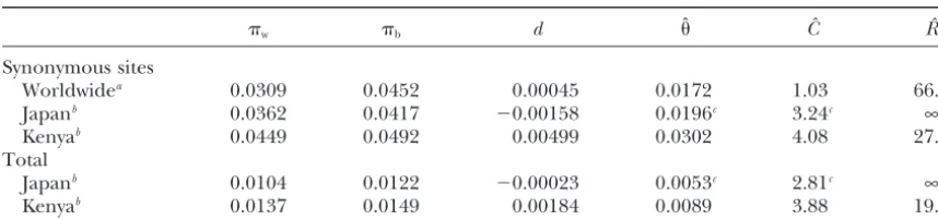
TABLE 1

Estimates of␪,C, andRof theAmymultigene family inD. melanogaster

␲w ␲b d ␪ˆ Cˆ Rˆ

Synonymous sites

Worldwidea _{0.0309 0.0452 0.00045 0.0172 1.03 66.6}

Japanb _{0.0362 0.0417 ⫺0.00158 0.0196}c _3.24c _∞

Kenyab _{0.0449 0.0492 0.00499 0.0302 4.08 27.2}

Total

Japanb _{0.0104 0.0122 ⫺0.00023 0.0053}c _2.81c _∞

Kenyab _{0.0137 0.0149 0.00184 0.0089 3.88 19.0}

a_{Data fromInomataet al.(1995).} b_{Data fromArakiet al.(2001).}

c␪_{andCwere estimated assumingR}⫽∞_.

as␲w,␲b, anddare calculated from DNA sequence data. different loci on the same chromosome are identical, andc2is the probability that two alleles from different For theAmygenes ofD. melanogaster, given␲w⫽0.0309,

␲b⫽ 0.452, and d ⫽ 0.000452, the minimum xis ob- loci from different chromosomes are identical. These identity coefficients are written in terms of the amounts tained when␪ ⫽0.0172,C⫽1.03, andR⫽66.6.

Unfor-tunately, it is not possible to evaluate the variances of of variation considered here. That is, f ⫽ 1 ⫺ E(hw) andc1 ⬇ c2 ⬇ 1 ⫺ E(hb). Ohta (1982) obtained the these estimates. They might depend on␪,C,R, and the

sample size (n). Recombination within each gene may approximate expectations of three allelic identity coef-ficients using transient equations with the assumption decrease the variances.

that mutation, gene conversion, and recombination rates are small. In this study, the exact solutions for DISCUSSION _{m⫽K⫽2 were obtained without this assumption by a}

diffusion method. This method is useful to obtain the A simple two-locus gene conversion model was

consid-variances ofhw,hb, andD. The transient equations for ered to investigate the amounts of DNA variation and

the second orders of the identity coefficients are too linkage disequilibrium in small multigene families. The

complicated to solve (Ohta 1985; Basten and Weir

exact solutions for the expectations and variances of

1990). the amounts of variation within and between two loci

Using the theoretical results, a method for estimating were obtained. It was shown that gene conversion

in-the mutation, gene conversion, and recombination pa-creases the amount of variation within each locus and

rameters was developed. The method was applied to that the degree of increase is large when the gene

con-the data of con-theAmymultigene family ofD. melanogaster

version rate is relatively small. On the other hand, gene

(Inomataet al.1995). The estimate of␪for synonymous conversion decreases the amount of variation between

sites is 0.0172, which is close to the average of this species two loci and there is almost no difference between␲w

(0.0135;MoriyamaandPowell1996). The gene con-and␲bwhen the gene conversion rate is very large. The

version rate is estimated to beⵑ60-fold larger than the effect of recombination on the amounts of variation

estimate of the mutation rate for synonymous sites. The within and between two loci is relatively small. The

ex-amount of variation within a locus is much larger than pectation and variance of the amount of linkage

disequi-␪because of a high rate of gene conversion. librium were also obtained. Gene conversion generates

Similar results are obtained from recent data of the positive linkage disequilibrium and the degree of

link-same region (Table 1). Araki et al. (2001) reported age disequilibrium decreases as the recombination rate

sequence variations of theAmyregion in random sam-increases.

ples from Japan and Kenya. For the Kenyan sample,␪ The model considered here is a special case ofOhta’s

for synonymous sites and for the total coding region (1982) general model, and the theoretical results

ob-are estimated to be 0.0302 and 0.0089, respectively. C

tained in this article are consistent with her results.

for the total coding region is estimated to be 3.88, which

Ohta (1982) considered an intrachromosomal gene

is similar to that for synonymous sites (4.08). The simi-conversion model of multigene families withKalleles,

larity of the two estimates of C is consistent with the where the number of loci is assumed to be constant

mechanism of gene conversion, because a single conver-(m). Her model with m ⫽ K ⫽ 2 corresponds to the

sion event usually involves a certain length of DNA frag-model of this study.Ohta(1982) investigated the three

ment. For the Japanese sample, since negatived is ob-identity coefficients,f,c1, andc2, at equilibrium.fis the

served, the estimation was conducted assuming free probability that two alleles sampled from the same locus

Figure2.—Linkage disequilibrium in theAmy

genes inD. melanogaster.

to those of the Kenyan sample. An estimate of ␪ for no variation is observed when selection is very strong (H. Innan,unpublished results).

synonymous sites is about fourfold bigger than that for

the total coding region, while two estimates of C are _{The author thanks M. Nordborg for comments. This study was} similar. Estimates of␪andCfor the Kenyan sample are supported in part by a fellowship from the Japan Society for the

Promotion of Science.

larger than those for the Japanese sample, probably because of the difference of population size.

To estimate␪,C, andR, these parameters are assumed

to be constant across the region. The obtained estimates LITERATURE CITED

might be the averages for all the sites considered. Since _{Araki, H., N. InomataandT. Yamazaki,2001 Molecular evolution} theAmygenes ofD. melanogasterare reversely duplicated, of duplicated amylase gene regions in Drosophila melanogaster: evidence of positive selection in the coding regions and selective Rcould have a large heterogeneity across the region.

constraints in thecis-regulatory regions. Genetics157:667–677.

Assuming the recombination rate per site is constant _{Bahn, E.,1967 Crossing over in the chromosomal region}

determin-ing amylase isozymes in Drosophila melanogaster. Hereditas58: (␳per kb),Rfor the first position isⵑ4.5␳and for the

1–12.

last position isⵑ7.5␳ because the length of the region

Baltimore, D.,1981 Gene conversion: some implications for

immu-between the two Amy genes is ⵑ4.5 kb. The effect of _{noglobulin genes. Cell24:592–594.}

Basten, C. J.,andB. S. Weir,1990 Effect of gene conversion on

heterogeneity in the recombination rate on␦was

investi-variances of digenic identity measures. Theor. Popul. Biol.38: gated (Figure 2) because the effect ofRon␦is relatively _125–148.

large. Almost no correlation was detected, suggesting Birky, Jr., C. W.,andR. V. Skavaril,1976 Maintenance of genetic homogeneity in systems with multiple genomes. Genet. Res.27: that the effect of the heterogeneity ofRon the estimates

249–265.

may not be large. _{Black, J. A.,andD. Gibson,1974 Neutral evolution and} immuno-The method considered here ignores the effect of globulin diversity. Nature250:327–328.

Dover, G.,andE. Coen, 1981 Springcleaning ribosomal DNA: a

selection, and estimates might be biased if selection

model for multigene evolution? Nature290:731–732.

is working. Purifying selection decreases the amounts of _{Edelman, G. M.,andJ. A. Gally,1970 Arrangement and evolution} variation within and between two loci. The effect of se- of eukaryotic genes, pp. 962–972 inNeurosciences: Second Study Program, edited byF. O. Schmitt.Rockefeller University Press,

lection is large and complicated when some kind of

New York.

balancing selection acts to maintain two different alleles _{Inomata, N., H. Shibata, E. OkuyamaandT. Yamazaki,1995} Evo-in a population. The amount of variation between two lutionary relationships and sequence variation of␣-amylase vari-ants encoded by duplicated genes in theAmylocus ofDrosophila

loci increases dramatically as selection intensity

in-melanogaster.Genetics141:237–244.

creases. The amount of variation within each locus is _{Kimura, M.,1964 Diffusion models in population genetics. J. Appl.}

Probab.1:117–232.

Moriyama, E. N.,andJ. R. Powell,1996 Intraspecific nuclear DNA _{because E(p}3₎ ⫽ _E(q)3_{, E(p}2_q) ⫽ _E(pq2_{), and E(pD)}⫽ variation inDrosophila.Mol. Biol. Evol.13:261–277.

E(qD). From (A1–A3), we have the solutions forE(p3_), Nagylaki, T.,1984a Evolution of multigene families under

inter-E(p2_{q), andE(pD). To show the solutions, it is helpful} chromosomal gene conversion. Proc. Natl. Acad. Sci. USA81:

3796–3800. _{to introduce the equations}

Nagylaki, T.,1984b The evolution of multigene families under

intrachromosomal gene conversion. Genetics106:529–548. _{GA⫽ ⫺2⫺2␪ ⫺C, GB⫽ ⫺6⫺6␪ ⫺2C⫺R, GC⫽2C⫹2C}2_⫹6␪C,

Nagylaki, T.,andT. D. Petes,1982 Intrachromosomal gene

con-version and the maintenance of sequence homogeneity among GD⫽CE(p2_{)⫹CE(pq)⫹(2⫹ ␪)E(D), GE⫽ ␪E(p}2_{)⫹2(1⫹ ␪)E(pq),} repeated genes. Genetics100:315–337.

Nei, M.,andA. K. Roychoudhury, 1974 Sampling variances of HA⫽ ⫺4C⫺CGB, HB⫽ ⫺(2⫹ ␪)CE(p2_)⫺GAGD, heterozygosity and genetic distance. Genetics76:379–390.

Ohta, T.,1976 Simple model for treating evolution of multigene HC⫽ ⫺CGD⫺CGE, HD⫽ ⫺C2_⫹ CGA,

families. Nature263:74–76.

Ohta, T.,1977 On the gene conversion model as a mechanism for IA⫽GCHB⫺HCHD, IB⫽ ⫺HAHD⫺GAGBGC.

maintenance of homogeneity in systems with multiple genomes.

Then,E(p3_),E(p2_{q), andE(pD) are given by} Genet. Res.30:89–91.

Ohta, T.,1978 Theoretical population genetics of repeated genes forming a multigene family. Genetics88:845–861.

E(p3₎⫽GD

C ⫹

HC GC

⫺ GBIA

CIB

⫺HAIA

GCIB

, (A4)

Ohta, T.,1981 Genetic variation in small multigene families. Genet. Res.37:133–149.

Ohta, T.,1982 Allelic and nonallelic homology of a supergene

family. Proc. Natl. Acad. Sci. USA79:3251–3254. E(p2_q)⫽ ⫺HC GC

⫹HAIA

GCIB

(A5)

Ohta, T., 1983 On the evolution of multigene families. Theor. Popul. Biol.23:216–240.

and

Ohta, T.,1984 Some models of gene conversion for treating the evolution of multigene families. Genetics106:517–528.

E(pD)⫽ ⫺IA

IB

. (A6)

Ohta, T.,1985 Variances and covariances of identity coefficients of a multigene family. Proc. Natl. Acad. Sci. USA82:829–833. Ohta, T.,andM. Kimura,1969a Linkage disequilibrium due to

In a similar way, we have the following six equations

random genetic drift. Genet. Res.13:47–55.

lettingg⫽p4_,p3_q,p2_q2_,p2_{D,pqD, andD}2_: Ohta, T.,andM. Kimura,1969b Linkage disequilibrium at steady

state determined by random genetic drift and recurrent

muta-⫺(3⫹ 2␪ ⫹C)E(p4₎⫹_CE(p3_q)⫹₍₃⫹ ␪_)E(p3₎⫽_0,

tion. Genetics63:229–238.

Payant, V., S. Abukashawa, M. Sasseville, B. F. Benkel, D. A. _(A7) Hickeyet al., 1988 Evolutionary conservation of the

chromo-somal configuration and regulation of amylase genes among eight

CE(p4_{)⫺(6⫹8␪ ⫹4C)E(p}3_q)⫹3CE(p2_q2_)⫹6E(p2_D) species of theDrosophila melanogasterspecies subgroup. Mol. Biol.

Evol.5:560–567.

⫹ ␪E(p3₎⫹₍₆⫹₃␪_)E(p2_q)⫽_{0, (A8)}

Shibata, H.,andT. Yamazaki, 1995 Molecular evolution of the duplicatedAmylocus in theDrosophila melanogasterspecies

sub-group: concerted evolution only in the coding region and an _4CE(p3_{q)⫺(4 ⫹8␪ ⫹4C)E(p}2_q2_)⫹8E(pqD) excess of nonsynonymous substitutions in speciation. Genetics

141:223–236. _{⫹ (4⫹4␪)E(p}2_{q)⫽0, (A9)}

Smith, G. P.,1974 Unequal crossover and the evolution of multigene families. Cold Spring Harbor Symp. Quant. Biol.38:507–513.

2E(p2_q2_)⫺4CE(p2_{D)⫹8E(pqD)⫺(6⫹8␪ ⫹4C⫹2R)E(D}2₎

Smith, G. P.,1976 Evolution of repeated DNA sequences by unequal crossover. Science191:528–535.

Walsh, J. B.,1988 Unusual behaviour of linkage disequilibrium in ⫺4E(p2_q)⫺₍₈⫺_4C)E(pD)⫹_2E(pq)⫹_2E(D)⫽_{0, (A10)}

two-locus gene conversion models. Genet. Res.51:55–58.

⫺CE(p4_)⫺CE(p2_q2_{)⫺(12⫹8␪ ⫹4C⫹R)E(p}2_{D)⫹2CE(pqD)}

Communicating editor:F. Tajima

⫹CE(p3_)⫹

CE(p2

q)⫹(6⫹2␪)E(pD)⫽0, (A11)

and APPENDIX

⫺2CE(p3_q)⫹ _2CE(p2_D)⫺ ₍₁₀⫹₈␪ ⫹_4C ⫹_R)E(pqD)

In equilibrium, lettingg⫽ p3_,p2_{q, and pDin (2) and}

⫹ 2E(D2₎⫹_2CE(p2_q)⫹ ₍₄⫹₂␪_)E(pD)⫽_{0. (A12)} (6), we have three equations for E(p3_{), E(p}2_{q), and}

E(pD), _{From (A7–A12), we have the solutions of equilibrium}

⫺(6⫹6␪ ⫹3C)E(p3_)⫹3CE(p2_{q)⫹(6⫹3␪)E(p}2_)⫽0,

expectations forp4_,p3_q,p2_q2_,D2_,p2_{D, andpqD.To show} (A1) the very complicated solutions, it is helpful to introduce

the following equations: CE(p3_{)⫺(2⫹6␪ ⫹C)E(p}2_{q)⫹4E(pD)⫹ ␪E(p}2_{)⫹2(1⫹ ␪)E(pq)⫽0,}

(A2)

JA⫽3⫹4␪ ⫹2C, JB⫽ ⫺1⫺2␪ ⫺C, and

JC⫽ ⫺12⫺8␪ ⫺4C⫺R, JD⫽ ⫺3⫺4␪ ⫺2C⫺R, ⫺CE(p3₎⫺_CE(p2_q)⫺₍₆⫹₆␪ ⫹_2C⫹_R)E(pD)⫹_CE(p2₎

JE⫽ ⫺3⫺2␪ ⫺C, JF⫽ ⫺10⫺8␪ ⫺4C⫺R,

KC⫽ ⫺2E(p2_{q)⫺(4⫺2C)E(pD)⫹E(pq)⫹E(D), YC⫽MG/MF⫺MDYA/MFYB,}

KD⫽CE(p2_{q)⫹(2⫹ ␪)E(pD), KE⫽(1⫹ ␪)E(p}2_{q)/C, ZA⫽YA/YB, ZB⫽LBYA/LAYB, ZC⫽CLFYC/LA.} LA⫽ ⫺2C3_{⫺2CJAJB, LB⫽ ⫺2C}3_{⫺4CJA, LC⫽C}2_JE⫹C2_JB,

Then,E(p4_{), E(p}3_q),E(p2_q2_),E(D2_),E(p2_{D), andE(pqD)} are given by

LD⫽ ⫺CKA⫺CKB, LE⫽2C⫺2CJBJD, LF⫽ ⫺6C⫺CJC, LG⫽ ⫺4C⫺2CJD, LH⫽2C2_⫺2C2_{JE, LI⫽C(8⫺JDJF)⫺4CJD,}

E(p4₎⫽_M

I⫺2ZA⫺ZB⫺ZC⫹

KA⫺JCYC

C , (A13)

LJ⫽ ⫺C2_{(3⫹ ␪)E(p}3_{)⫺CJEKA, LK⫽ ⫺2C(1⫹ ␪)JAE(p}2_q)⫹CLD,

E(p3_{q)⫽ ⫺K} E⫹

2ZA⫹JB(MI⫺ZB⫺ZC)

C , (A14)

MA⫽LA[C2_{(1⫹ ␪)E(p}2_q)⫹LJ],

MB⫽CLA[2KC⫺2JDKD⫺2(1⫹ ␪)JDE(p2_q)],

E(p2_q2_{)⫽ ⫺M}

I⫹ZB⫹ZC, (A15)

MC⫽C(LALG⫺LELF), MD⫽LALH⫺LBLC, ME⫽LALI⫺LBLE,

E(D2_{)⫽ ⫺K}

D⫺CKE⫹CYC⫹2ZA⫹

JFZA

2 ⫹JB(MI⫺ZB⫺ZC), (A16) MF⫽ ⫺C(LCLF⫹JCJELA), MG⫽MA⫺LCLK,

E(p2_{D)⫽ ⫺Y}

C, (A17)

MH⫽MB⫺LELK, MI⫽LK/LA,