Physiologically Based Model Development and Parameter Estimation: Benzene Dosimetry in Humans and Respiratory Irritation Response in Rodents

(1)

YOKLEY, KAREN ALYSE Physiologically Based Model Development and Parameter Es-timation: Benzene Dosimetry in Humans and Respiratory Irritation Response in Rodents. (Under the direction of Professor H.T. Tran).

One can form mathematical equations based on a combination of chemistry, physics, and biological information to represent a physiological system. Once a model is formulated based on the physiological system, we must make sure that the inputs or parameters to the model also faithfully represent the system. In this study, we adapt and combine existing mathematical models to describe different physiological systems.

(2)

observed human population variability.

(3)

by

Karen Alyse Yokley

A dissertation submitted to the Graduate Faculty of North Carolina State University

in partial satisfaction of the requirements for the Degree of

Doctor of Philosophy

Applied Mathematics with a Concentration in Computational Mathematics

Raleigh 2005

Approved By:

Dr. Paul Schlosser Dr. James Selgrade Committee Member Committee Member

(4)

(5)

Biography

(6)

Acknowledgments

First of all, I would like to thank my committee. I would like to thank my advisor, Dr. Hien Tran, for support and encouragement throughout my graduate work. I am very grateful for his understanding and patience. I am also thankful to Dr. Paul Schlosser who motivated the problems in this study and was a great source of knowledge on modeling and in biology. I would also like to acknowledge Dr. Mette Olufsen and Dr. James Selgrade for research and professional advice.

Many thanks to CIIT Centers for Health Research for support via a fellowship. I greatly appreciate the insight and knowledge of Annie Jarabek (U.S. EPA), Dr. Mel Anderson, and all others who collaborated on both the benzene and irritant projects. I would like to also thank Dr. Fred Miller, a long-term supporter of respiratory modeling including the project in Chapter 3. I would also like to acknowledge Kaija Pekari and Stephen Rappaport for sharing data and ideas. The research described in Chapter 2 was supported in part by a grant from the National Institute of Environmental Health Sciences (P30ES10126).

I would also like to thank Dr. Ralph Smith for encouraging me to stick with graduate school when I had difficulty with my qualifying exams. Many people in the math department also provided encouragement throughout my time at North Carolina State, especially Brenda Currin, Rory Schnell, Lesa Denning, and Denise Seabrooks.

(7)

I want to thank Molly McNeeley for dealing with my insanity. Thanks to Molly, Katie Kavanagh Fowler, and Vicky Williams Klima for the many girls’ nights that were necessary to make it through. I’ll never think of Twin Peaks, V, or Iron Chef without being reminded of you. Thanks also go out to Beth Kirsch, Ushma Shukla, and Scott and Diana Padgett. I really appreciate all the stress-relieving racquetball matches with Nick Luke and Rich Schugart. Thanks also to fellow graduate students Dewey Taylor, Jill Reese, Jeff Hood, Rachel Levy, Brian Adams, Brandy Benedict, Jason Osborne, and Karen Bliss.

(8)

List of Figures

2.1 Schematic description of the benzene model. . . 10

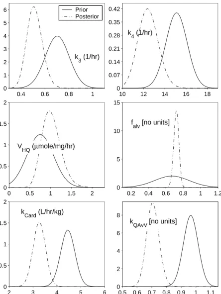
2.2 Prior distributions plotted alongside posterior distributions for six of the investigated parameters. . . 18

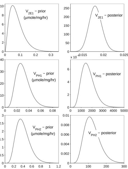
2.3 Prior distributions and posterior distributions for three of the investigated parameters. . . 19

2.4 The model predictions versus data for benzene in exhaled air with higher exposure levels from [71]. . . 20

2.5 The model predictions versus data for benzene in blood with higher exposure levels from [71]. . . 21

2.6 The model predictions versus data for benzene in exhaled air with lower exposure levels from [71]. . . 21

2.7 The model predictions versus data for benzene in blood with lower exposure levels from [71]. . . 22

2.8 The model predictions versus metabolite data from [82]. . . 23

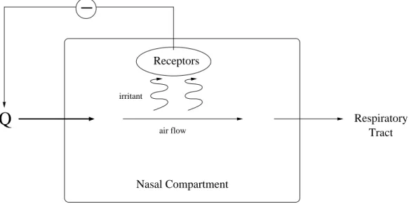
3.1 Brief illustration of the sensory response to irritants. . . 33

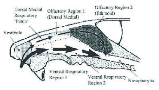
3.2 Illustration of the rat nasal anatomy. . . 34

3.3 Schematic of model simplification. . . 37

3.4 An example of a control functionxsteady. . . 44

3.5 Plot of pseudo-steady-state solution for ventilation Q(t) in the presence of formaldehyde. . . 73

3.6 Plot of pseudo-steady-state values for ventilation Q(t) in the presence of formaldehyde versus inhalation concentration. . . 73

3.7 The solutions to the model for the concentration of the irritant in various compartments, the solutions for the firing rate in various compartments, and the solutions for ventilation while varying the parameterτr. . . 80

3.8 The solutions to the normalized sensitivity equations of the compartmental concentrations, the firing rates, and the ventilation rates to changes in τr. . 81

(11)

concentrations, the firing rates, and the ventilation rates to changes in k0. . 83 3.11 The solutions to the model for the concentration of the irritant in various

compartments, the solutions for the firing rate in various compartments, and the solutions for ventilation while varying the parameterτQ. . . 84

3.12 The solutions to the normalized sensitivity equations of the compartmental concentrations, the firing rates, and the ventilation rates to changes in τQ. . 85 3.13 The solutions to the model for the concentration of the irritant in various

compartments, the solutions for the firing rate in various compartments, and the solutions for ventilation while varying the parameterp. . . 86 3.14 The solutions to the normalized sensitivity equations of the compartmental

concentrations, the firing rates, and the ventilation rates to changes in p. . . 87 3.15 The solutions to the model for the concentration of the irritant in various

compartments, the solutions for the firing rate in various compartments, and the solutions for ventilation while varying the parameterα. . . 88 3.16 The solutions to the normalized sensitivity equations of the compartmental

concentrations, the firing rates, and the ventilation rates to changes in α. . 89 3.17 The solutions to the model for the concentration of the irritant in various

compartments, the solutions for the firing rate in various compartments, and the solutions for ventilation while varying the parameterKD. . . 90

3.18 The solutions to the normalized sensitivity equations of the compartmental concentrations, the firing rates, and the ventilation rates to changes in KD . 91

3.19 The graph of the inhalation exposure studies from [25]. . . 92 3.20 Solution for ventilation for 7.8 ppm exposure using parameters optimized

over only this data set. . . 99 3.21 Solution for ventilation for 13.7 ppm exposure using parameters optimized

over only this data set. . . 99 3.22 Solution for ventilation for 27.5 ppm exposure using parameters optimized

over only this data set. . . 101 3.23 Solution for ventilation for 7.8 ppm exposure after using five parameters from

the optimization from only the second data set and optimizing over τr and τQ2. . . 102

3.24 Solution of ventilation for 27.5 ppm exposure after using five parameters from the optimization from only the second data set and optimizing over τr and τQ2. . . 102

3.25 Solution of ventilation for the 7.8 ppm exposure after optimizing over only

τQ with fixed values from an optimization over the second data set and an

averaged value of τQ2. . . 103

averaged value of τQ2. . . 104

(12)

List of Tables

2.1 Fixed parameters used in the PBPK model [28]. . . 11 2.2 Partition coefficients used in the PBPK model [28]. . . 12 2.3 Prior distributions for the PBPK model parameters analyzed using the Markov

Chain Monte Carlo Method. . . 15 2.4 The resulting distributions for the PBPK model parameters from the Markov

Chain Monte Carlo Method. . . 17 2.5 The sensitivity analysis results for each investigated parameter. . . 22 3.1 Values of fixed parameters used in the respiratory portion of the sensory

irritant model. . . 48 3.2 Values of fixed parameters used in the sensory response portion of the sensory

irritant model. . . 48 3.3 Beginning values for the parameters in the sensitivity analyses. . . 76 3.4 Resulting values from a least squares minimization on the first data set. . . 98 3.5 Resulting values from a least squares minimization on the second data set. . 100 3.6 Resulting values from a least squares minimization on the third data set. . . 100 3.7 Resulting values for two parameter optimizations with the 7.8 ppm and 27.5

(13)

Chapter 1

Introduction

Modeling of physiological systems can incorporate many different methods and perspectives. Mathematical equations based on a combination of chemistry, physics, and biological information, inevitably using simplifying assumptions, can be derived to represent a physiological system. These representations may elucidate more about the physiological system than experimentation alone and allow one to extrapolate from quantitative exper-imental data to predict results for situations where we have no data. Although various mathematical approaches exist for modeling biological systems, we specifically will consider models described by differential equations.

One way to model chemical distribution throughout the body is through compart-mentalization. If we look at an animal’s body as composed of compartments (of tissues, organs, groups of organs, etc.), we can simplify how we consider the amount of chemical in the body as a whole. Hence, we can formulate equations only describing where a chemical is in a portion of the nasal cavity or in the blood flow to the kidneys. This way, we can better describe the local concentration of a chemical and further understand how that chemical is causing its effects in different parts of the body. For examples of models incorporating chemical movement through compartments, see [8, 20, 22, 29, 28, 36, 39] although [20] does not contain explicit equations. In order to model the flow of chemicals through the body, we must also consider mode of transport.

(14)

from one area to another as a result of random molecular motion [64]. As stated in [34], diffusion can be described using Fick’s law and a diffusion coefficient, or it can be explained in terms of a mass transfer coefficient. Basically, both methods contain the same idea of diffusion, but sometimes it is easier to convey the derivation of a model using one set of terminology than with the other. Let us first consider Fick’s Law of Diffusion and then extend the law to the idea of a mass transfer coefficient. Fick’s Law states that the rate of diffusion of a gas across a fluid membrane is (1) proportional to the difference in partial pressure, (2) proportional to the area of the membrane, and (3) inversely proportional to the thickness of the membrane [1]. Mathematically, Fick’s Law for the one-dimensional case is described

J =−D∆C(t)

∆x ,

whereJ is the particle flux (mass flow rate per unit area across which diffusion is occurring),

C is the concentration of the solute,Dis the diffusion coefficient,x is the distance into the substrate (i.e., the membrane), andtis the diffusion time [2, 3]. If we consider the movement in terms of across a cross-sectional area (i.e., surface area of the membrane), we can consider

dM

dt =−DA

∆C

∆x,

whereM is the mass of substrate in the compartment from which mass is flowing andAis the interfacial area across which the substrate flows [4]. Knowing the concentration gradi-ent, i.e., using the replacement ∆C=C1−C2, we can rewrite the above equation

dM1

dt =− DA

∆x(C1−C2),

(15)

dM1

dt =−K(C1−C2).

K can be thought of as a mass transfer coefficient. As described in [34], we expect that the amount of chemical transfered is proportional to concentration difference across the interface and the area of that interface, i.e.,

N1=k(c1i−c1), (1.1)

whereN1 is the flux at the interface into the compartment, c1i is the concentration at the

interface, andc1 is the the concentration in the bulk solution. In Chapter 3, we will formu-late a model for sensory irritant response beginning with a transport model from [39]. We will not go into an entire derivation of this model, but we will demonstrate from a basic example how either Fick’s Law or the idea of a mass transfer coefficient can be used in the model formulation. The model description in [39] begins with mass transport, modeled

N =Kg(Cg−Cl/P), (1.2)

where

N = flux from gas to liquid phase (µmol/[cm2×h])

Kg = overall mass transfer coefficient (cm/h) Cg = concentration in gas phase (µmol/cm3)

P = the liquid:air partition coefficient (dimensionless)

Cl = concentration in liquid phase (µmol/cm3).

(16)

p=KCl,

whereprepresents partial pressure of the gas andKrepresents Henry’s law constant for that particular substance. (Partial pressure is simply a measure of the gas-phase concentration in different units.) Note that the K above is not the same K in the definitions of Fick’s Law mentioned earlier. Taking a section from [70],

Henry’s law is applicable to layers of biological fluids and tissues. In this situa-tion, the ratio at equilibrium of the concentrations in the two phases or layers is the ratio of the Henry’s law constant of the air/solution system of one phase to the Henry’s law constant of the air/solution system of the other phase. This ratio is called the “distribution coefficient” or “partition coefficient.”

Returning to the flux equation, note that (1.2) is formulated as is (1.1) with mass transport coefficient k = Kg. Also note that in Chapter 3 we will use this same idea to model the loss of chemical to the rat nasal cavity wall assuming that the chemical concentration in the cavity wall is zero (or c1i = 0). Further, in addition to the incorporation of Fick’s

Law in the model in Chapter 3, a simpler “flow in - flow out” formulation based on fluid flow from compartment to compartment is used in both the models discussed in Chapters 2 and 3 and listed in Appendices A and B. Movement by concentration gradient is not incorporated in the model in Chapter 2 and Appendix A, and that model is considered to be completely flow-limited. The flow-limited formulation of the model in Chapter 2 is assumed to be sufficient to describe the physiological system. We should note that care was taken to remove the spacial variable in the original formulation of that model from [28] and extended in Chapter 2. The liver was considered as three separate compartments in the benzene model so that the model would remain an ordinary differential equation system and be entirely flow-limited. Additionally, the description of flow through the nasal cavity in the model from [39] and adapted in Chapter 3 is also based on a “flow in minus flow out” formulation. We recognize that modeling in terms of concentration gradient is necessary for some situations, but we hope to capture enough of the chemical transport to faithful represent the physiological system through only fluid flow in the benzene model in Chapter 2.

(17)

nasal cavity surface area (as in Chapter 3) may be relatively easy to find, but parameters involved in changes within the body, such as chemical reaction rates, may be more difficult to access. Using optimizations methods with the model and experimental data, the parameters which give the best fit of the model to the data can be found as in [28] and as in Chapter 3. If, however, we want to incorporate variability across a population and have distributions instead of fixed values for certain parameters, other methods involving sampling can be used. We incorporate Bayesian methods in Chapter 2 to accomplish such a goal.

Several different iterative optimization algorithms exist, most of which can be de-scribed as gradient-based algorithms or deterministic sampling algorithms. One gradient based algorithm is the steepest descent method which updates the current iteration by the formula

x+=xc−λ∇f(xc),

where λ is a chosen steplength and f(x) is the function to be minimized [55]. Note that for our purposes ∇f(x) would be partial derivatives with respect to the parameters be-ing estimated, i.e., the sensitivity equations. Hence, the steepest descent method should be easy to implement if the sensitivity equations are known. If the sensitivity equations and their solutions are easily available, gradient-based methods work very quickly and very well. Sensitivity equations, however, can be tedious to obtain and may take time to solve numerically within the gradient-based optimization. If many parameters are being esti-mated, i.e., if many sensitivity equations are necessary to establish the gradient, choosing a deterministic sampling method may be better. Some deterministic algorithms include the Nelder-Mead simplex algorithm and the DIRECT algorithm. The Nelder-Mead algorithm keeps a simplex S of approximations to an optimal point. The N + 1 vertices are then ordered according to the function values

f(x1)≤f(x2)≤ · · · ≤f(xN+1).

(18)

Multidi-rectional Search algorithm. These algorithms are slower than gradient based methods but require no sensitivity equations. The algorithm DIRECT is also a sampling algorithm, but it incorporates the division of the parameter space into hyper-rectangles or hyper-cubes in order to find the solution that produces the minimum [38, 55]. The algorithm DIRECT can be very helpful if reasonably small bounds are known for the estimated parameters. If a large parameter space is being searched, DIRECT can be very slow. All of these methods or a combination of these methods can be used in estimating the best fixed parameters for mathematical models.

Although the model presented in Chapter 3 is a model for rats, the overall intention of the formulation models of chemical exposure is to eventually better understand risk to humans. Modeling of the biological system presented in Chapter 3 is at an early stage, but the investigation of sensory irritation will hopefully lead to a model related to humans. Therefore, at this stage it makes sense to only be concerned with the optimization of fixed parameters and not to overly complicate the model. At some point, we could incorporate variability in parameters as in the model as in the model in Chapter 2. An older and more established model is extended to incorporate human variability in Chapter 2. Since the population of humans is so diverse, having constant parameters that indicate rates of reactions and cardiac flow for the entire population does not take many factors into consideration. Humans have different physiologies dependent on such things as age, sex, and diet as well as more subtle genetic differences. By looking at a few parameters as distributions in Chapter 2 we hope to capture some of the overall variability in benzene metabolism. We will use the Markov Chain Monte Carlo Method as is further explained in Section 2.2 to find distributions for investigated parameters for the established model from [28].

(19)

Chapter 2

Physiologically Based

Pharmacokinetic (PBPK)

Modeling of Benzene in Humans:

A Bayesian Approach

2.1 Introduction

(20)

metabolism, and elimination through the body can assist in the assessment of acceptable levels of exposure.

Physiologically based pharmacokinetic (PBPK) models are standard tools that are now often used in risk assessment to better extrapolate from experimental animals to humans and from high to low exposures [46, 23]. In [29], the authors developed a PBPK model that predicts tissue concentrations of benzene and its key metabolites in mice using metabolic parameters obtained in vitro. The PBPK model tissue compartments include the liver, richly perfused and poorly perfused tissues, and adipose tissue. Two additional compartments, the stomach and the alveolar gas-exchange region, were also included to describe oral and inhalation exposures, respectively. This model was later extended to take into account the zonal distribution of enzymes and metabolism in the liver, rather than treating the liver as one homogeneous compartment [28]. A common characteristic of PBPK models, such as the model in [28], is that they have single-valued parameters and are deterministic.

However, when the PBPK models are extended to humans, accounting for the multiple sources of variability that will affect dosimetry in humans is important. This hierarchy of variances includes variability among: different studies, individuals within each study, and measurements taken from each individual. To properly account for the variability at any of these levels PBPK models should be integrated into a statistical framework that acknowledges these sources of variation.

(21)

predictions and allowing them to vary can result in better model predictions than keeping them fixed, just as fitting the volume of distribution in classical pharmacokinetic models provides the flexibility to fit most data. One may question, however, whether this flexibility results in a model that is more predictive of the population as a whole and if it masks other errors in model specification. Because of these concerns and questions, one might wish to perform analyses that treat physiological parameters as fixed while updating distributions for metabolic parameters, for which prior information is much weaker and which are known to vary considerably among individuals. In order to capture variability of these physiolog-ical parameters, we use Bayesian analysis to fit PBPK model parameter to sets of human data.

In this study, the Monte Carlo simulation program MCSim [18] was used to fit a PBPK model of benzene to sets of human data by performing a series of simulations along a Markov chain in the model parameter space. We hypothesized that the observed inter-individual variability resulted primarily from known or estimated variability in key metabolic parameters and that a statistical PBPK model that explicitly included variability in only those metabolic parameters (along with any known variation in body weight) would be sufficient to describe all observed variability. The result of MCMC fitting of the model to data produces samples from the Bayesian posterior distribution of the model parameters.

2.2 Materials and Methods

(22)

Liver Liver Liver 1 3 2 Fat Slowly Perfused Kidney Rapidly Perfused BENZENE Lung Blood Alveolar Space Kidney Fat _PerfusedSlowly _PerfusedRapidly

Blood PMA Stomach MA Arterial Blood Venous Blood GST GST CYP2E1 CYP2E1 GST GST EH Kidney Fat _PerfusedSlowly _PerfusedRapidly

Blood Liver Liver Liver 1 3 2 Kidney Fat _PerfusedSlowly _PerfusedRapidly

Blood

Liver

Liver Liver

1

3 2

BENZENE OXIDE PHENOL HYDROQUINONE

PH Conjugates HQ Conjugates Catechol THB Inhaled Exhaled CYP2E1 CYP2E1 CYP2E1 CYP2E1 Sulfation Glucuronidation CYP2E1 Liver Liver Liver 1 3 2 Liver Liver Liver 1 3 2 Liver Liver Liver 1 3 2 Fat Slowly Perfused Kidney Rapidly Perfused BENZENE Lung Blood Alveolar Space Kidney Fat _PerfusedSlowly _PerfusedRapidly

Blood

Fat _PerfusedSlowly _PerfusedRapidly

Blood PMA Stomach MA Arterial Blood Venous Blood GST GST CYP2E1 CYP2E1 GST GST EH Kidney Fat _PerfusedSlowly _PerfusedRapidly

Blood

Blood Liver Liver Liver 1 3 2 Liver Liver Liver 1 3 2 Kidney Fat _PerfusedSlowly _PerfusedRapidly

Blood

Blood Liver Liver Liver 1 3 2 Liver Liver Liver 1 3 2

BENZENE OXIDE PHENOL HYDROQUINONE

PH Conjugates HQ Conjugates Catechol THB Inhaled Exhaled CYP2E1 CYP2E1 CYP2E1 CYP2E1 Sulfation Glucuronidation CYP2E1 Liver Liver Liver 1 3 2 Liver Liver Liver 1 3 2

Figure 2.1: Schematic description of the benzene model from [28].

data used in this study is inhalation data, the parameter k8, the rate of uptake from the stomach to the liver, and the equation (A.27) have no effect on our solutions.

Total cardiac flow, QCard, and alveolar ventilation, QAvV, were assumed to be

proportional to body weight and to each other. These values were defined by

QCard = kCard·BW QAvV = kQAvV ·QCard,

and the proportionality constants kCard and kQAvV were left for later investigation. The

(23)

Table 2.1: Fixed parameters used in the PBPK model [28]. Parameter Value Unit Source

QL 0.2370QCard L/h [35] QF 0.0425QCard L/h [35] QK 0.2027QCard L/h [35] QS 0.1717QCard L/h [35] QR 0.3461QCard L/h [35]

VL 0.025BW L [50]

VF 0.1429BW L [35]

VK 0.004BW L [35]

VS 0.734BW L [50]

VR 0.040BW L [50]

VBl 0.07429BW L [35]

CCP _14.5 _mg/g _[32]

CM P 58 mg/g [32]

K_m,P H₁ 1.4 µM [78]

K_m,P H₂ 220 µM [78]

KmHQ 746 µM [78]

ABZ 0.0397 1/µM [63]

AP H 1.30·10−2 1/µM [63]

AHQ 10−7 1/µM [63]

k1 4.20·10−2 L/µmol [63]

k2 32.16 1/h [63]

k5 4.00·10−2 L/µmol [63]

k6 2.13·10−3 L/µmol [63]

k7 2.03·10−4 L/µmol [63]

k8 374.9598 1/h [28]

k9 0.1163 1/h [28]

k10 0.1443 1/h [28]

QCard =QF +QS+QR+QL+QK. (2.1)

Partition constants P_BlBZ_:_Air, P_jBZ, and P_jBO (for compartments j = fat, liver, slowly per-fused tissue, rapidly perper-fused tissue, and kidney) were also changed to the values in [20] because those values were thought to better represent human values. The values for the concentration of microsomal protein per gram of tissue in the liver, CM P_{, and the}

concen-tration of cytosolic protein per gram of tissue in the liver, CCP_{, were changed from the}

(24)

Table 2.2: Partition coefficients used in the PBPK model [28]. Parameter Value Source

P_BlBZ_:_Air 7.80 [20]

P_FBZ,P_FBO 54.50 [20]

P_LBZ,P_LBO 2.95 [20]

P_SBZ,P_SBO 2.05 [20]

P_RBZ,P_RBO,P_KBZ,P_KBO 1.92 [20]

P_FP H 27.63 [60]

P_LP H 2.17 [60]

PP H

S 1.22 [60]

PP H

R ,PKP H 2.17 [60]

P_FHQ 4.06 [60]

P_LHQ 1.04 [60]

P_SHQ 0.94 [60]

P_RHQ,P_KHQ 1.04 [60]

to be relatively invariant between species; hence the remaining parameters in the PBPK model are unchanged from their values in [28]. In addition, the PBPK model has equations describing the cumulative amount of exhaled benzene and in order to compare the model to data of the concentration of exhaled benzene, the following expression was used to compute the model value for concentration of benzene in exhaled air

C_EBZ = (1−falv)·CIBZ+falv

£

QCard·

¡

CVBZ−CABZ¢

+QAvV ·CIBZ

¤

/QAvV. (2.2)

The notation from the original model is preserved in (2.2) with the only new value being

falv, which is the fraction of each inhaled breath that perfuses the alveolar space. This

equation is essentially identical to a correction used by [53] and is derived by assuming that: air leaving the alveolar region satisfies the usual venous-equilibration model; air leaving the alveolar space mixes with air that was inhaled but only entered the physiological dead space (conducting airways; DS); that the DS air does not exchange with blood at all and hence stays at the inhaled concentration; and that the measured exhaled concentration is the result of this mixture. Thus the exhaled concentration equals falv times the concentration

exiting the alveolar region plus (1−falv) times the DS concentration that equals the inhaled

concentration. The value forfalv was expected to be around 0.67 [50] and was investigated

(25)

prediction of the amount of urinary metabolite was divided by a standard value of urinary excretion as converted from 20 ml/kg/day to compute the predicted concentration over time [27].

To illustrate the statistical considerations, suppose that a multivariate PBPK model for benzene can be specified by the n-dimensional system of differential equations

dx

dt =f(t, x, q), x(t0) =x0 t0= 0. (2.3)

The solution to this system of equations denoted byg(t, q, x0) is a function of parametersq (including inhalation exposure conditions), timet, and initial condition x0. Now, consider the case ofin vivo data collected on each of m subjects exposed to benzene. Each of these subjects are assumed to follow the basic model (2.3), but with potentially different param-eters and initial conditions, reflecting variation in pharmacokinetic paramparam-eters across the population. Although analysis of individual subject data provides insight into underlying biology, it fails to address the broader issue of how these parameters vary across individu-als. Comprehensive application of PBPK models to these data requires that both levels of inquiry, individual and population, be addressed–not only to elucidate individual-specific parameter values but also to characterize the extent and nature of their variation across population.

Formally, for individuali, with intermittent observations available at time ti1,ti2,

. . . tin, let Yij = (Yi1j, Yi2j, , Yimj)T be the (m×1) vector of observations on subject i at

time tij; for example, Yij may include measurements of benzene in blood and expired air.

Thus, data collected on individualiare the vectorsYij,j = 1,2, . . . , nj, ideally assumed to

be observations on the system (2.3). However, the measurements of benzene concentration in the exhaled air, benzene concentration in the blood, and metabolite amounts in the urine are subject to several sources of variation. To specify this explicitly, we may specify the individual statistical model

Yij =g(tij, qi, xi0) +²ij, j= 1,2, . . . , ni, (2.4)

(26)

model due to the combined effects of these sources at time tij, and qi and xi0 are the parameters and initial conditions specific to individuali. Notice that the quantity of interest here is the distribution of parametersqi.

The modified PBPK model was implemented into Fr´ed´eric Bois’ and Don Maszle’s Monte Carlo simulation program, MCSim, which uses Metropolis-Hasting sampling for its Markov Chain Monte Carlo simulations [18]. Markov Chain Monte Carlo simulations were run on the model in order to find distributions of specific metabolic parameters that had been held constant in the previous PBPK modeling studies [28]. The model parameters investigated included V2E1, the CYP2E1 specific activity as determined by the oxidation of p-nitrophenol to p-nitrocatechol; VP H1 and VP H2, the maximum rates of metabolism of phenol by two sulfate transferases; and VHQ, the maximum rate of conjugation for

hydro-quinone (primarily glucuronidation). The two first order rates of metabolism of benzene oxide into phenylmercapturic acid and into muconic acid,k3 and k4, respectively, were also expected to be distributed and so were incorporated into the MCSim program. The values forkCard,kQAvV, andfalv were likewise expected to be distributed and were analyzed using

MCSim.

The prior distributions for V2E1,VP H1, VP H2, and VHQ were determined by

ana-lyzing previous in vitro data obtained from human liver samples [78]. The initial rates of phenol sulfation and rates of hydroquinone glucuronidation from the in vitro study were each multiplied by factors yielded by the mathematical model used in [78]. The factors were 0.18 forVP H1, 2.4 for VP H2, and 11.1 for VHQ. The CYP2E1 activity measurements

were not multiplied by a factor. These vectors of data were converted to proper units then entered in Matlab. These four vectors were tested to see if they fit a normal, uniform, gamma, or Poisson distribution. The best fitting distribution for each parameter, i.e., the hypothesized distribution that was not rejected and had the highest p-value, was used as its prior. The parameters V2E1,VP H1, and VP H2 were expected to have gamma distributions based on the in vitro data, and the model parameter VHQ was expected to be normally distributed. Since little information was available on the other investigated parameters, the remaining priors were based on previous constant values. The prior distributions fork3 and

k4 were assumed to be normally distributed, and the means of these priors were the fixed values from the original mouse model [28]. The priors for kCard,kQAvV, and falv were also

(27)

Chain Monte Carlo Method.

Parameter Prior Distribution

k3 Normal,µ= 0.7032, σ= 0.1

k4 Normal,µ= 15.1001,σ = 1

V2E1 Gamma,a= 2.7506, b= 0.0284

VP H1 Gamma,a= 6.8926, b= 0.0044

VP H2 Gamma,a= 6.8926, b= 0.0585

VHQ Normal, µ= 0.7484, σ= 0.3207 falv Normal,µ= 0.67, σ= 0.2 kCard Normal,µ= 4.4571, σ= 0.3 kQAvV Normal,µ= 0.965, σ= 0.05

the distributional components for each of these model parameters, and the specific prior distributions used in the simulations are contained in Table 2.3.

Data taken from previous studies of human benzene exposure were incorporated into the MCSim program, and extra specifications were used in the case of multiple data sets for the same individual in order to find inter-individual variability as opposed to intra-individual variability. In one study, blood and exhaled air samples were collected from three healthy nonsmokers who were each exposed to four hour periods of both 10 cm3/m3 and 1.7 cm3_/m3 _{benzene [71]. Thirty-five occupationally exposed individuals provided urine} samples during their work shifts for metabolite data in a second study [75, 82]. Even though the time length of their shifts and the urine collection times varied, the exposure time for these workers was taken to be six hours in the model. The Markov Chain Monte Carlo simulation was run for 20,000 iterations, and the results were recorded every tenth iteration. The results were analyzed from iteration 15010 through 20000 in order to ascertain the distributions of the model parameters.

(28)

changed from 0.1 to 0.3 and from 0.01 to 0.05, respectively. After this change, theMCSim

program was run again. Only one long run was assumed to be sufficient as suggested in [43] although Bois and Maszle believe considering several pooled runs is a better approach [18]. After the posterior distributions were determined, the model was examined for sensitivity. The means of each posterior distribution were used for the investigated param-eters to produce solutions from the model. In order to ascertain the model’s sensitivity to each parameter, one parameter would be varied while all the other investigated parameters were kept at the mean values from their posterior distributions. For each investigated pa-rameter, three solutions were produced holding the other eight of the parameters at their distributional means and then using a value at 95% of the confidence interval, a value at 5% of the confidence interval, and the mean of the currently analyzed parameter. Then the maximum distance from the mean solution to the solution above or below the mean curve was computed and used in the following formula

sensitivity= ∆prediction/prediction

∆parameter/parameter. (2.5)

In the above formula,predictionindicates the predicted solution at the mean and ∆prediction

indicates the maximum difference between the predicted solution at the mean and the pre-dicted solution using either a 95% or 5% confidence interval value. The values in the denominator of the above ratio are based on the varying investigated parameter and are defined similar to the predicted solutions. The only state variables of the model examined for sensitivity were those compared to data in this study in order to better understand which data sets influenced the results of each investigated parameter.

2.3 Results

The output fromMCSimappeared to sample adequately from the posterior distri-butions and was analyzed using Matlab to find distridistri-butions which best fit the output data for each parameter. These posterior distributions for the nine investigated model parame-ters are shown in Table 2.4 as well as compared graphically to their priors in Figure 2.2 and Figure 2.3. ForkCard the mean,µ, and the standard deviation,σ, of its normal distribution

(29)

Chain Monte Carlo Method.

Parameter Posterior Distribution

k3 Gamma, a= 63.8027, b= 8.060·10−3

k4 Gamma,a= 170.74,b= 0.07282

V2E1 Gamma, a= 140.58, b= 1.286·10−4

VP H1 Gamma,a= 7.310, b= 225.53

VP H2 Gamma,a= 7.8377, b= 15.5516

VHQ Gamma,a= 20.2275, b= 0.05037 falv Beta, a= 169.29,b= 65.7663 kCard Normal, µ= 3.2635, σ= 0.2634 kQAvV Gamma, a= 276.63, b= 2.557·10

−3

are listed for falv. For the other parameters the resulting shape parameter, a, and inverse

scale parameter, b, of the gamma distributions are given. The values for k3 and k4 are slightly below those found in the optimization with the mouse model [28], and the posterior distributions for the metabolic rates VP H1 and VP H2 allow for much higher values than in

vitro data [78] would suggest. The posterior distribution for V2E1 has moved to the left

within its prior distribution, which was based on the in vitrodata from [78]. Although the prior ofVHQ is normal and its posterior distribution appears to be a gamma distribution, the values of this parameter have changed little through the use of MCMC. The values for

kCardandkQAvV are slightly below their priors, which were based on reference mean values.

The posterior distribution forfalv is narrower than its prior, but the mean of the posterior

is slightly higher than the mean of the prior.

One hundred solution curves were computed from the 100 samples from theMCSim

(30)

0.4 0.6 0.8 1 0

1 2 3 4 5 6

k 3 (1/hr)

Prior Posterior

10 12 14 16 18 0

0.07 0.14 0.21 0.28 0.35 0.42

k 4 (1/hr)

0 0.5 1 1.5 2 0

0.5 1 1.5 2

V

HQ (µmole/mg/hr)

0.2 0.4 0.6 0.8 1 1.2 0

5 10 15

f

alv [no units]

2 3 4 5 6 0

0.5 1 1.5 2

k

Card (L/hr/kg)

0.5 0.6 0.7 0.8 0.9 1 1.1 0

2 4 6 8

k

QAvV [no units]

(31)

0 0.1 0.2 0.3 0

2 4 6 8 10

V

2E1 − prior (µmole/mg/hr)

0.015 0.02 0.025 0

50 100 150 200 250

V

2E1 − posterior

0 0.02 0.04 0.06 0.08 0

10 20 30 40

V

PH1 − prior (µmole/mg/hr)

0 1000 2000 3000 4000 5000 0

2 4 6

x 10−4

V

PH1 − posterior

0 0.2 0.4 0.6 0.8 1 1.2 0

0.5 1 1.5 2 2.5 3

V

PH2 − prior (µmole/mg/hr)

0 100 200 300 0

0.002 0.004 0.006 0.008 0.01

V

PH2 − posterior

(32)

0 0.2 0.4

10−4 10−2 100

Subject 1

0 0.2 0.4

Benzene Concentration (

µ

mol/L)

10−4 10−2 100

Subject 2

0 10 20 30 40 50 0

0.2 0.4

0 10 20 30 40 50 10−4

10−2 100

Subject 3

prior posterior

−−−

Time (h)

Figure 2.4: The model predictions versus data for benzene in exhaled air with higher expo-sure levels from [71].

73 kg for subject 3.

One hundred samples for each model parameter were drawn from the distributions found throughMCSim, and 100 model solutions were computed using these parameters for different exposures using Matlab. The 100 solution values for different metabolites in the urine were plotted in Figure 2.8 versus the corresponding data values from the occupational exposure study [75, 82]. Each vertical line of x’s represents the 100 predicted exhaled benzene concentrations (µmoles/L) for the model for a particular inhalation concentration plotted versus an actual measurement from the study. A plot of they =xline is contained in all parts of Figure 2.8 for comparison. All five metabolite solutions seemed somewhat centered around the y=x line except for the plot of the catechol and trihydroxy benzene concentration.

(33)

0 1 2

10−2 100

Subject 1

0 1 2 3

µ

mol/L)

10−2 100

Subject 2

0 10 20 30

0 1 2 3

0 10 20 30

10−2 100

Subject 3

Time (h) prior −−−

posterior −−−

Figure 2.5: The model predictions versus data for benzene in blood with higher exposure levels from [71].

0 0.02 0.04 0.06

10−4 10−2

Subject 1

0 0.02 0.04 0.06

µ

mol/L)

10−4 10−2

Subject 2

0 5 10 15 20 25

0 0.02 0.04 0.06

0 5 10 15 20 25

10−4 10−2

Time (h)

Subject 3

prior ₋₋₋

posterior ₋₋₋

(34)

0 0.1 0.2 0.3 0.4

10−2 10−1 100

Subject 1

0 0.1 0.2 0.3 0.4

µ

mol/L)

10−2 100

Subject 2

0 5 10 15 20 25

0 0.1 0.2 0.3 0.4

Time (h)

0 5 10 15 20 25

10−2 100

Subject 3

prior

posterior −−−

−−−

Figure 2.7: The model predictions versus data for benzene in blood with lower exposure levels from [71].

Table 2.5: The sensitivity analysis results for each investigated parameter.

k3 k4 V2E1 VP H1 VP H2 VHQ falv kCard kQAvV

MA 2.07 1.65 2.20 6.9·10−4 0.058 0.21 0 2.30 4.40 Cat-THB 1.66 2.00 2.18 5.6·10−4 0.014 0.13 0 1.51 3.89 PMA 0.99 2.04 1.98 5.9·10−4 0.015 0.17 0 2.33 4.23 PH 2.40 0.86 2.58 7.8·10−4 0.020 0.23 0 6.33 3.91 HQ 0.59 0.91 1.47 2.1·10−4 0.0053 0.67 0 0.69 1.51

C_EBZ (high) 2.03 3.90 2.24 2.3·10−6 3.2·10−6 4.2·10−5 1.94 3.21 3.09

C_EBZ (low) 0.089 1.56 2.01 5.0·10−6 2.4·10−5 1.7·10−7 1.94 4.55 3.63

CABZ₊_CVBZ _(high) _2.03 _3.90 _2.24 ₂_.₃_·₁₀−6 ₃_.₂_·₁₀−6 ₄_.₂_·₁₀−5 ₀ _3.21 _3.15

CABZ₊_CVBZ _(low) _0.089 _1.56 _2.01 ₅_.₀_·₁₀−6 ₂_.₄_·₁₀−5 ₁_.₇_·₁₀−7 ₀ _4.55 _3.60

two exposure levels from [71].

2.4 Discussion

(35)

hy-0 100 200 300 400 500 600 700 800 900 1000 0

500 1000 1500

MA

0 100 200 300 400 500 600 700 800

0 200 400 600 800

Cat−Thb

0 20 40 60 80 100 120

0 50 100 150

PMA

predicted

0 500 1000 1500 2000 2500 3000 3500 4000

0 2000 4000 6000

PH−conj

0 50 100 150 200 250 300 350 400 450 500

0 2000 4000 6000

HQ−conj

actual

(36)

droquinone conjugates, and the model greatly under-predicts the concentrations of catechol and trihydroxy benzene for the workplace data [75, 82]. Since Bayesian methods depend greatly on the accuracy of prior information, errors in the data used to estimate the priors could account for the need to alter theMCSimoutput for a better fit graphically. The model seems to predict the concentration of benzene exhaled and the concentration of benzene in blood well for the study in [71] although a wider range of solution curves capturing all data points was expected. Although the computed solutions using the posterior distributions do not greatly improve accuracy over the solutions computed using the prior distributions for this study, the range of posterior model solutions does narrow somewhat around the expo-sure data. Since the two studies probably varied in participant physical activity, further experiments focusing on activity levels might help the accuracy of the model.

The results forfalvhave a mean around 0.72, which is slightly higher than the ILSI

value of 0.67 [50], but the presence of benzene may have increased the subjects’ ventilation rates. Measurements of the dead space lung volume of subjects exposed to butadiene suggest that it lowers the dead space to around 171.3 mL[61], which is around 14.6% of the total lung volume [35]. Our results suggest that the dead space lung volume does decrease with inhaled benzene but only to about 28% of total volume. However, in the study from [71], the apparatus for sampling exhaled air may have introduced a slight source of error due to the difficulty to breathe normally. The three subjects may have unconsciously breathed with larger tidal volumes thus decreasing the relative dead space volume. Also, while it is normally assumed that no gas exchange occurs in the conducting airways, a small amount almost certainly occurs; and the larger falv could simply allow the model to correct for the

fact that it only allows exchange in the alveolar space.

A significant portion of the data used in this investigation involved benzene con-centrations in blood and exhaled air. In the PBPK model [28], the amount of benzene exhaled depends directly on the parameters QAvV,QCard, andPBlBZ:Air. We have quantified QAvV and QCard as being proportional to kCard and kQAvV, respectively, and introduced

the parameter falv for the fraction of inhaled air perfusing the alveolar region. Although

the equation describingAMBZ

E is connected to the rest of the ordinary differential equation

system, the model dynamics of the exhaled concentration of benzene are therefore most closely related to the parameters falv, kCard, kQAvV, and the concentration of benzene in

(37)

the liver, particularly V2E1. The results of the sensitivity analysis in Table 2.5 show that

falv,kCard,kQAvV, andV2E1, as well as k3 and k4 (rate constants for conversion of benzene

oxide to phenylmercapturic acid and muconic acid, respectively), affect the exhaled ben-zene. (An increase ink3 ork4 reduces the amount benzene oxide which would otherwise be converted to phenol, and hence the amount of phenol competing with benzene for CYP2E1.) Not surprisingly, these same parameters, exceptfalv, also significantly affect the predicted

concentration of benzene in blood.

Since the predictions of benzene concentrations in exhaled air and in blood depend most strongly onk3,k4,V2E1,falv,kCard, andkQAvV,MCSimwould primarily be able affect

the fit of the model to the exhalation and blood data by updating the distributions of these particular six parameters. Hence, the posterior distributions found by MCSim for k3, k4,

V2E1,falv,kCard, andkQAvV were largely influenced by the process of fitting solution curves

to the exhalation and blood data. Likewise, since changes in falv only alter the exhaled

benzene predictions, only the exhalation data affects the falv posterior distribution in the

MCMC simulations. The model does not seem to be very sensitive to changes in VP H1,

VP H2, and VHQ, although the effect is slightly higher when dealing with the metabolites.

The sensitivity of model predictions for urinary metabolite concentrations to changes ink3,

k4,V2E1,VP H1,VP H2,VHQ,kCard, andkQAvV suggests that the data from the occupational

study influences the distributions estimated for all investigated parameters except for falv.

When the model prediction of one output variable is less sensitive to a particular parameter, theMCSimprogram will be more influenced by the data of other output variables (that do show greater sensitivity) when finding the posterior distribution of that particular parameter. Hence, the effect the urinary metabolite data has on the distributions ofVP H1,

VP H2, andVHQ is less than the occupational study data has on other parameters and is less

significant than the effect the blood and exhalation data have on most other parameters. Further, any miscalculation due to the apparatus used by [71] will significantly affect our results for falv, and use of the data from [75, 82] cannot significantly compensate for such

(38)

When both the mathematical model and the statistical model are fully specified at all levels, the approach is referred to as a parametric approach. Specifically in the PBPK model, the approach is considered parametric when assuming a distribution form (e.g., log-normal) for how well we know each individual’s parameters and a distribution form for the set of parameters from all the individuals. A parametric approach is often used when the general form of the distribution in the problem is known. A statistical model is considered to be structured when the variables (distributions) are associated with specific underlying quantities, which occurs naturally with PBPK model. A parametric approach provides an efficient way for estimating the parameters of a PBPK model since it takes full advantage of the distribution structure.

A variety of statistical tools are available for fitting the mathematical models to data with structured variability. Model-fitting tools that do not incorporate prior informa-tion on parameter distribuinforma-tions, referred to as ”frequentist,” include maximum likelihood methods such as non-linear least squares [14]. The error structure in the data (how sources of error or variability are assigned) can be accommodated by modifying standard tech-niques to incorporate ideas from repeated measures and cross-over experimental designs. Alternatively, Bayesian statistical models provide a natural framework for analyzing mod-els with hierarchical error structures [40]. One Bayesian technique that has been embraced by a great many applied statisticians in all fields of research is the Markov chain Monte Carlo (MCMC) method [44]. MCMC methods explore the joint posterior distribution of interest (i.e., the distribution of all parameters, given that the distributions may not be independent) by providing a mechanism whereby a set of realizations or samples from that distribution can be generated. This set is obtained by carrying out Monte Carlo simulations from a Markov chain that is constructed so that its stationary distribution is the relevant posterior. Various methodologies exist to carry out the required simulations including the Gibbs sampling algorithm and the Metropolis-Hastings algorithm. Because of the increasing complexities of statistical models encountered in practice, MCMC provides a much-needed unifying framework within which many complex problems can be analyzed.

(39)

significant contributions in the field of PBPK modeling. In [17] Bayesian statistical inference and physiological modeling were brought together to model the distribution and metabolism of benzene in humans. This approach of combining PBPK models and MCMC methodology for Bayesian inference has been extended to other chemicals such as toluene and styrene [52, 53]. The inclusion of the variability predicted by these approaches into risk assessments is expected to be an improvement over previous use of empirical uncertainty factors (e.g., [62]).

In [17], Bois also applied Bayesian analysis to a PBPK model of benzene in humans using the data of [71], which is also included in our analysis. The paper of Bois and co-workers was one of the first to demonstrate the application of Bayesian analysis to PBPK modeling and its use in predicting population variability, a significant advancement in the potential for mechanistic dosimetry modeling in risk analysis. The model used by Boiset al. in [17], however, only included a very simple description of benzene metabolites, with the assumption that phenolic metabolites are a fixed fraction of those metabolites. That model does not allow for prediction of target tissue concentrations of phenol itself (as opposed to phenol conjugates), nor of hydroquinone or benzene oxide, both of which are included in our model. Hydroquinone and phenol have been shown to strongly synergize in the induction of genotoxicityin vivo[12] and hydroquinone was shown to strongly enhance colony formation of murine bone marrow cellsin vitro[51]. Benzene oxide has been shown to be tumorigenic in mice [21], and benzene exposure-related increases in benzene oxide-albumin adducts have been demonstrated in humans [72, 73]. Thus we believe the current model builds upon and is a considerable advancement of the innovative work by Bois and colleagues in that it predicts tissue levels of phenol, hydroquinone, and benzene oxide, all of which are likely contributors to benzene’s leukemogenic effects. Further, the current results are based on a much larger data set than that used in the previous analysis, providing for more robust and representative posterior distributions.

(40)

seemed possible. Therefore we decided to test the hypothesis that the observed variability in the data would be accounted for by incorporating distributions for only the metabolic parameters by fixing the values of most physiological variables to standard values used in PBPK modeling (e.g., [50]) and the measured partition coefficients to those measured or estimated elsewhere.

Incorporation of dependence on activity level and variability and uncertainty in partition coefficients would almost certainly have resulted in much closer correlations be-tween predictions and the data. Hence activity considerations should probably be added before the benzene PBPK model is used in a human risk assessment, but we believe there is scientific value in first testing this more stringent assumption presented here. While we do not know precise activity levels for the individuals whose data are being simulated here, the authors of [52] found the best description of their data for toluene when ”the increased perfusion of peri-renal fat was set to a constant level during all exercise levels,” which indi-cates that categorical assignment of values based on general activity patterns (e.g., resting, some movement, light work, etc.) would be sufficient.

(41)

mousein vivo data.

Thus we could potentially ”correct” the over-prediction of the [15] data and [82] data by updating k9 and k10. If we had allowed those parameters to be updated better fits probably could have been obtained without further insight. Instead the failure of the model to fit the data given the constraints of holding those parameters constants led us to the possibility that we had over-predicted the rate of uptake by inhalation. Benzene has a blood:air partition coefficient of 7.8 [20]. While this is relatively low and benzene has low aqueous solubility, one might expect a limited wash-in/wash-out effect that would lower absorption from the amount predicted by the classic venous ventilation model used here [42]. After this analysis, we decided not to use the data from [15] in our study rather than alterk9 ork10 or the blood:air partition coefficient. In addition to not utilizing the Berlin data, we did update the cardiac flow and alveolar ventilation rate through the parameters

kCard and kQAvV. After the decision to neglect the data from [15] in our analysis, k9 and

k10were investigated briefly through the MCMC method using priors based on values from [28]. The intention was to improve the results with catechol and tryhydroxy benzene, but no significant improvement resulted in the fit to data from either the [71] study or the occupational data from [75, 82].

The difference between a model adjustment by increasing the macromolecule bind-ing constants and decreasbind-ing predicted inhalation rates is potentially significant because the latter would result in a reduction in the prediction of total phenol and hydroquinone pro-duction and hence in potential target tissue dosimetry of active metabolites. Future work on benzene PBPK modeling for humans should probably first seek to implement a more anatomically accurate inhalation model, such as those described by [77, 33] before updating the macromolecule binding constants. If after making such structural changes to eliminate model bias the predicted pharmacokinetic distributions still do not cover the data, we would then have greater support for including other sources of variability and possibly updating their distributions as well.

(42)

(43)

Chapter 3

Sensory Irritation Response in

Rats

3.1 Introduction

Airborne irritants, such as formaldehyde, ozone, and chlorine, are capable of stimu-lating trigeminal nerve endings in the mucosa of the respiratory tract of rodents [6, 7, 13, 59]; and the presence of these chemicals can cause a painful burning sensation [6]. Stimulation of these endings has been shown to decrease respiratory frequency, increase tidal volume, and decrease overall respiratory minute volume in the rat [37] and in mouse neonates [81]. Formaldehyde, on which we will particularly focus, has been shown to be carcinogenic in rodents and is found in the environment as a result of both anthropogenic and natural mechanisms [24].

(44)

prior to the data collection [26]. Both studies showed a recovery in respiration after the exposure period ended.

Studies of the effects of inhaled irritants have often involved air flow and how the chemicals are deposited in the nasal cavity. In [56, 57, 58], studies focused on air flow simulations to predict formaldehyde deposition. Connections were made between fluid dynamic modeling and formaldehyde carcinogenicity in rats in [31]. By looking at flux and chemical disposition, researchers can better predict irritant effects. Modeling the flow disposition of inhaled irritants as in [8, 39, 41] can also aid in the understanding of responses to these chemicals.

In order to best model the overall decrease in minute ventilation due to inhaled irritants, we should incorporate the effects of the trigeminal stimulation as well as the air flow of the chemical through the respiratory tract. Many gases, such as formaldehyde and ammonia, are absorbed rapidly in the upper respiratory tract [48]; and hence, we must incorporate some loss of chemical to the nasal cavity walls in our assessment of chemical location. By considering the sensory activity in response to the presence of irritant in addition to modeling the flow of chemicals through the respiratory tract, we hope to better model the effects on respiration than by directly connecting exposure level to ventilation decrease.

(45)

Nasal Compartment

Q

Respiratory

Tract

irritant

Receptors

air flow

Figure 3.1: Brief illustration of the sensory response to irritants. Qrepresents the ventilation rate which decreases due to the receptor activity in the presence of irritant.

3.2 Sensory Irritant Model Formulation

3.2.1 Upper Respiratory Model

(46)

Figure 3.2: Illustration of the rat nasal anatomy divided into compartments corresponding to the epithelium lining the lumen. This illustration was taken from [39] where it was modified from its version in [65].

• Air flows consisted of the following:

1. all inhaled air flowing across the nasal vestibule

2. – dorsal medial air stream flowing over respiratory epithelium then olfactory epithelium

– a second composite ventral and lateral air stream flowing over the remaining respiratory epithelium (divided into anterior and posterior compartments) 3. all air then recombining and passing over a nasopharynx compartment

4. air then entering a composite lower respiratory tract compartment

• The olfactory region of rodents was divided into a small dorsal anterior compart-ment and a large compartcompart-ment representing the remaining olfactory epithelium on the septum and ethmoid turbinates.

(47)

mucus phase, (3) epithelial phases, and (4) a blood exchange region. In addition to consid-ering the vapor in these phases, the model included a differential equation for the amount of chemical in the mucus buffer. Hence, for each compartment, the model has a system of at least five ordinary differential equations. The first equation for each compartment is the air phase:

Vair dCair

dt = Q(Cair−in−Cair)

−KgcSc(Cair−[X[nonionized]Cmuc/Pmuc:air]),

where

Cair = concentration of non-ionized vapor exiting air compartment (µmol/cm3) Cair−in = concentration of non-ionized vapor entering air compartment (µmol/cm3)

Cmuc = total concentration of vapor (ionized & non-ionized) in the

mucus layer (µmol/cm3)

X[non−ionized] = fraction of vapor present in non-ionized form (dimensionless)

Pmuc:air = mucus:air partition coefficient of the non-ionized acid (dimensionless) Vair = volume of air compartment (cm3)

Sc = surface area of compartment c (cm2)

Vair = volume of air in the compartment (cm3)

Kgc = compartmental mass transfer coefficient (cm/s) Q = the air flow in (and out) of the compartment (cm3/s).

(48)

• The model from [39] includes five compartments in the nasal passageway, a dorsal respiratory compartment, two dorsal olfactory compartments, and two ventral respi-ratory compartments. We considered only using three nasal compartments–one dorsal respiratory compartment, one dorsal olfactory compartment, and one ventral respira-tory compartment, but since most similar models do keep all five compartments we decided to be consistent with the other models. See Figure 3.3.

• We are not as concerned with the damage to the tissue in the nasal cavity or details of disposition within the tissue as we are with the overall nasal absorption and transfer of formaldehyde. Therefore we can simplify the removal of vapor from the air phase to a single loss term. Also see Figure 3.3.

• Since the current model will not track formaldehyde chemistry within the mucosa, the concentration of mucus buffer can be ignored and so we will not use this equation in our system at this time.

We can begin the model adaption to our system by looking at the first differential equation in the hybrid CFD-PBPK model that describes the concentration of vapor in the air phase:

Vair dCair

dt =Q(Cair−in−Cair)−KgcSc(Cair−[X[nonionized]Cmuc/Pmuc:air]). (3.1)

The equation (3.1), subsequently altered for our model, could represent the air phase in each of our three respiratory compartments and two olfactory compartments. Since we are only concerned at this time with a loss to the mucosa we could rewrite this equation for the nasal vestibule and each of the five nasal passageway compartments as follows:

VN V dCN V

dt = Q(Cinh−CN V)−Kgc,N VSN VCN V (3.2) VV R1dCV R1

dt = fVQ(CN V −CV R1)−Kgc,V R1SV R1CV R1 (3.3) VV R2

dCV R2

(49)

mucosa mucosa Inspired

Air With Vapor

Nasal Vestibule Compartment

Respiratory Lower

Nasopharynx

Dorsal

Ventral

mucosa mucosa mucosa

R

O1

R1

R2

O2

(50)

VDRdCDR

dt = fDQ(CN V −CDR)−Kgc,DRSDRCDR (3.5) VDO1

dCDO1

dt = fDQ(CDR−CDO1)−Kgc,DO1SDO1CDO1 (3.6) VDO2

dCDO2

dt = fDQ(CDO1−CDO2)−Kgc,DO2SDO2CDO2, (3.7)

where our compartments are described by N V (the nasal vestibule), V R1 and V R2 (the ventral respiratory compartments), DR (dorsal respiratory compartment), and DO1 and

DO2 (dorsal olfactory compartments). The other terms are taken from the original model and are as follows:

Cinh = the concentration of formaldehyde being inhaled (µmol/cm3)

Ci = concentration of formaldehyde in the given compartment i (µmol/cm3) Si = surface area of compartment i (cm2)

Vi = volume of air in compartmenti (cm3)

Kgc,i = compartmental mass transfer coefficient for compartment i (cm/s) fV, fD = the fraction of inspired air that goes through the ventral

flow and through the dorsal flow, respectively,

fV +fD = 1 (dimensionless)

Q = the ventilation rate, i.e., the total air flow rate through the respiratory tract (cm3/s).

(51)

VN P dCN P

dt = Q(fDCDO2+fVCV R2−CN P)−Kgc,N PSN PCN P (3.8) VLRC

dCLRC

dt = Q(CN P −CLRC)−Kgc,LRCSLRCCLRC. (3.9)

Now, the notation is preserved from (3.2)-(3.7) withN P representing the nasopharynx and

LRCrepresenting the lower respiratory compartment, which should be clear pictorially from Figure 3.3. We should note that the equations shown in (3.8) and (3.9) are not necessary for the sensory response system we are considering, but they are included in the model formulation in case the lower respiratory tract requires focus in later work.

3.2.2 Nerve Response Control Equation

What remains is to describe our respiration rate (minute volume, although we will use different units), Q, in response to the irritant. We can get an initial model for nervous response by considering a model by J.T. Ottesen [69]. The study in [69] models the baroreflex-feedback mechanism which is the fastest control mechanism regulating human blood pressure. We are interested in this model because its description of the neurological control system could help us derive a control equation for the responses of nerves in the upper respiratory tract of rodents to inhaled irritants. The feedback model in [69] is evaluated using a simple model of the pulsatile cardiovascular system. The model of the feedback mechanism is divided into three parts: (1) the affector part, (2) the central nervous system part, and (3) the effector parts.

The first part of the model (the affector part) includes the part of the carotid sinus where the baroreceptors are located together with baroreceptor nerves. A change in carotid sinus arterial pressure causes deformation in the cross-sectional area of the sinuses (and hence the viscoelastic wall is deformed) which results in a change of activity of the baroreceptor nerves. This nerve activity is denoted as the firing rate; and the firing rate,

(52)

∆ ˙n1 = k1P˙c

n(M−n) (M/2)2 −

1

τ1

∆n1 (3.10)

∆ ˙n2 = k2P˙c

n(M−n) (M/2)2 −

1

τ2

∆n2 (3.11)

∆ ˙n3 = k3Pc˙ n(M−n) (M/2)2 −

1

τ3

∆n3, (3.12)

where n is the firing rate; M is the maximal firing rate; ˙Pc is the time derivative of the pressure at carotid sinus; and ∆n1, ∆n2, and ∆n3 denote the deviations from a normal, unstimulated valueN. More precisely,N is the steady-state firing rate that occurs with no pressure signal. The equations (3.10), (3.11), and (3.12) each describe the three different time-scale responses from the receptors in the baroreflex system, and hence each ∆ni

ex-presses the difference between the pressure-induced and time-dependent firing rate of that particular receptor and its normal firing rate Ni, i.e.,

∆ni =ni−Ni.

Our overall normal firing rate, N, and our total time-dependent firing rate, n, should be the sums of those values from the different receptor types; and hence, the solution to this differential equation system is such that

∆n1+ ∆n2+ ∆n3=

X

i ni−

X

i

Ni =n−N. (3.13)

Although the parameters ∆ni can be considered as physically representative, they can also