Robust Speaker Recognition for Large-scale
data using PFA Dimensionality Reduction
Rama Koteswara Rao P 1, Srinivasa Rao Y 2
Associate Professor, Department of Electronics and Communication Engineering, Sri Vasavi College of Engineering
and Technology, Nandamuru, Krishna Dt, India1
Professor, Department of Instrument Technology, AU College of Engineering, Visakhapatnam, AP, India2
ABSTRACT: This paper aims to improve the speaker recognition accuracy under noisy environments for large-scale
data set conditions. Performance of the recognition system mainly depends on feature extraction which extracts speaker specific information and the design of an efficient classifier. In this work, a factor dependent dimensionality reduction technique is employed to reduce the dimension of pitch and pitch strength based feature vectors, known as Principle Factor Analysis (PFA). A Voice Activity Detection (VAD) algorithm is applied to eliminate the background noise from the source utterance during the feature extraction phase. These features are useful in classification stage, where the identification is made on the basis of Support Vectors (SV) from the speaker database. FOLOS is the large-scale SVM algorithm, applied on the selected candidates that are PFA based dimensionality reduced feature vectors. The experimental results show that the proposed techniques give an improvement in recognition accuracy under noisy environments.
KEYWORDS:Principle Factor Analysis, Voiced Large Scale SVM, Pitched, Dimensionality Reduction, FOLOS.
I. INTRODUCTION
Since the dataset size of real-world speaker recognition systems is ever-increasing, large population speaker recognition systems pose challenges such as large training time, vast memory requirements and poor response time [1]. Though accuracy is the first consideration, robust recognition and adaptability are the significant aspects in real-world speaker recognition systems under large-scale dataset conditions. In previous work, good results have been achieved for the clean high-quality speech with matched training and test acoustic conditions. However, under mismatched conditions and noisy environments, often expected in real-world conditions, the performance of recognition systems degrades significantly, far away from the satisfactory level. Hence, robustness is a crucial research issue in speaker recognition systems. This motivates us to investigate new methods at various stages involved in typical speaker recognition systems.
Generic recognition system comprises of mainly two phases: training (also known as enrolment) and testing (classification) [2]. The enrolment stage extracts the speaker-specific information from speech signal in chronological mode to establish speaker models. A cluster of such models thereafter establishes the speaker database for later test phase. An anonymous speaker model is compared with the existing models in the database and then the results are expedited. In fact, feature extraction transforms the raw speech signal into a compact representation which is comparatively more stable and discriminative than the original signal [3]. In this work, effective methods have been proposed and experimental investigations have been carried out for the feature extraction, dimensionality reduction and classification phases.
the performance of these systems degrades severely under mismatched conditions and noisy environments. Hence, it necessitates deriving new set features for the speaker recognition under such conditions. From the previous evidences, it has been identified that the excitation source based features are less prone to environmental noise. Since the excitation source characteristics such as pitch and pitch strength exhibit the physiological and behavioral aspects of the speaker, good accuracy and lesser computational complexity can be achieved. This work mainly focus on feature extraction from the excitation source by accumulating characteristics from pitch and pitch strength of speech signal. In speaker recognition systems, large number of features increases the required memory and processing time. Hence,
dimensionality reduction becomes a crucial issue, which transfers a high-dimensional space into a space of fewer dimensions. In addition to the benefit of computational efficiency, it also improves the accuracy under mismatched conditions [9]. Principal factor analysis (PFA) is the most efficient and well studied projection, has been employed for dimensionality reduction in this work [14]. The proposers have conducted several investigations and performed the comparative analysis with respect to population size. Since these methods are successful in large-scale recognition tasks, original contributions are carried out in this work with respect to large-scale speaker recognition.
Verification is tested by Support Vector Machine (SVM), which is a successful discriminator and very effective method in the field of speaker recognition [15]. Specifically, SVM is employed in the context of statistical learning and thereby attributed to minimize the risk functions. However, the main constraints of the SVMs are its computational complexity and relatively poor performance under large-scale classification. In view of this, investigations for optimization of large-scale SVM algorithms have been carried. Large-scale SVM algorithm namely, FOLOS [18] has been identified with the combinations of different dimensionality reduction techniques. These approaches are very efficient for large datasets in typical classification domains such as pattern and speech recognitions.
The following section gives a brief description of Voice Activity Detection (VAD) algorithm. Section III describes the feature extraction from excitation source information. Section IV denotes the computation method, Principal Factor Analysis (PFA) dimensionality reduction technique. Section V briefly outlined FOLOS SVM training algorithm which is suitable to large-scale data. In section VI, the experimental results are summarized and made performance comparison. The last section concludes the findings and proposes the directions for future scope.
II. VOICE ACTIVITY DETECTION
Voice activity detectors (VAD) are used to separate the signal into non-speech segments and speech segments. Non speech segments are normally found from words silences, pre-utterance and post-utterance. Hence, algorithms are necessary to detect non-speech segments in a wide range of applications like speech recognition, speech coding, speech enhancement, etc. Specifically, VADs are required to adapt the changes in the noise characteristics for the estimation of non speech segments [10]. Since unvoiced segments are more similar to noise, it is very difficult to identify the unvoiced segments from speech signal. Unvoiced signals are generally lower SNR than voiced segments.
Voice activity detection process consists of the following two stages:
• Parameter extraction: Speaker-specific parameters are extracted from the speech signal. These extracted parameters have to show the discriminative variation between speech and non speech regions for the good quality detection. • Thresholding: A threshold is defined for the extracted parameters in order to divide the signal into speech and non-speech segments. This particular threshold should be adaptive or fixed.
A VAD for noisy conditions consists of parameter extraction stage, which is robust against a wide variety of noises and the thresholding methods are required to adapt the changes in noisy conditions.
2.1 Voice Detection from the entropy of magnitude spectrum
Energy based VADs furnish good performance when the energy of the speech signal is significantly greater than the energy of the background noise. When the SNR is very low (smaller than 0 dB), the energy of the background noise is similar to that of speech segments and thereby the detection by energy criterion provides poor results. However, speech regions are well organized in comparison with the noise regions when the observations are made from spectrograms. Specifically, Shannon’s entropy is an appropriate metric to measure the signal.
H(S) = −∑ ( ( ) log2 (P(s(i)))) (1)
Where, S = [s(1), .., s(i), ..., s(N)] represents a source of N symbols and the probability of emission P(s(i)) denotes for symbol i. If all the symbols are equi-probable (P (s(i)) = 1/N, ¥i), the entropy H(S) becomes maximal (H(S) = −log2( 1/N )), and becomes minimal (H(S) = 0) when the probability becomes one for at least one symbol.
The concept of speech detection is assumed that the speech signal is well organized during speech segments than noise segments. The entropy in the spectral domain is measured as:
(| ( , )| = − ∑Ω (| ( , )| ) ( (| ( , )| (2)
Where, | ( , )| = (| ( , )| )/ ∑Ω (| ( , )| is the probability function for the frequency band ω in the
magnitude spectrum.
Global statistics of the entropy of the signal is used to determine the threshold in this paper. This distribution is used by two Gaussian distributions to model and defined by using the expectation-maximization (EM) algorithm. These Gaussian distributions are used to determine the statistically optimal threshold. From Eq.(2), an adaptive method is used for the entropy.
H(|Y(t)|2) is maximum when Y becomes a white noise, H(X) = log(Ω), and minimum when it is a pure speech signal, H(Y ) = 0. The dynamics of H(.) is bounded by log() and 0 under white noise, thereby the entropy of the noise frame is not based upon the noise level. The entropy based method is best suited for the detection of white or quasi-white noises from the speech signal, but the performance is poor for colored noises. Speech segments can be detected by the thresholding of the entropy curve between the speech level and noise. The threshold value changes with the spectral nature of noise, but not when the noise level changes. As a result, VAD to be robust for the changes in the noise levels of the signals.
In case of colored noise, the entropy curve of non-speech regions is similar to the entropy of speech regions. In order to detect the entropy for the colored noise conditions, each frame of the spectrum is divided by the average spectrum. The entropy VAD is applied to the resulting spectrum which is similar to the white noise spectrum in non speech regions.
Ŷ( , ) = | ( , )|/ ∑ | ( , )| (3)
Where, | Ŷ (ω,t)| is the result of spectrum after whitening the filter. The speech regions can be detected from speech signal, but several variations are found in the noise segments. It is mainly due to the division by the average spectrum in Eq.(3), when the latter is smaller for different frequencies. In order to minimize this effect a white noise with small amplitude is mixed to the signal before computing the spectrum. As a result of this the speech regions are clearly detectable with the help of entropy.
III.FEATURE EXTRACTION
Pitch is the quality of sensation of frequency where all tones perceived by the listener are assigned to relative positions on the musical scale. Though sounds vary in pitch, some of the sounds have strong pitch sensation (e.g., vowels) whereas some do not (e.g., consonants). Accordingly, sounds are classified into pitched and non-pitched. Pitch information is valuable in speech applications such as music transcription, speech coding and query by humming [7]. As pitch differentiates the user’s speech appreciably, pitch and its strength are used as features for the proposed recognition system.
Let ( ); 0≤ ≤ −1 and 0≤ ≤ ( )−1, is the speech signal collected from different users, where be the number of users and ( ) be the number of samples taken from the user, provided, ( )= ( )= ( )=⋯=
. These samples become inputs for the feature extraction phase, where pitch and its strength are derived for each sample [6]. In feature extraction stage, continuous speech signals of all users are converted to discrete speech signals as
which each class has its own window size [8]. Afterward, the obtained windows of signal sequences are processed by the following Hanning window,
( ) = 0.5 1−
| | (4)
Where, 0≤ ≤| |−1, 0≤ ≤ −1,0≤ ≤ ( )−1, be the number of windows that belongs to kth class, wkl(m) is the mthinstant of time in lth window of kthclass and the parameters Wkl(m) are the Hanning coefficients derived from equation (4). The window size of each class is calculated as | | = 2 . A pitch vector [ ], ( )∈
{0,1} is generated with the size of Wkl(m), whereeach element is arbitrarily generated from {0,1} (i.e. ( )∈{0,1}). For each class of windows, centroids of pitched and non-pitched are derived as,
∑ ( ) ( )
∑| | ( ) ( ) (5)
∑ ( ) ( )
∑| | ( ) ( ) (6)
Where, ( ) is the magnitude of speech signal at a specific time interval indicated by the window element ( ). The time instant at which the pitch is present { } and the strength of pitch { }are determined as
{ } ={ ′}− and { } ={ ′}− respectively, where the sets{ ′} and { ′}are calculated as,
{ ′}≪ ;
( ( ) )
> 1
; ℎ
(7)
{ ′}≪ ( ); { }
; ℎ (8)
In (7), centroids ( and ) represent the maximum distance among centroid pairs. The centroids and are determined by firstly calculating the distance between each centroid pair as = − . Then, the parameters and contribute the maximum and are converted into and respectively. The obtained feature set { } and { }is stored as the first sample for the first user. The process is repeated for all samples of the same user and the obtained feature set is stored as feature matrix . Where, 0≤ ≤ ,0≤ ≤ −1, each column is composed of elements of feature set from each speech sample for a single user. Thus the obtained feature matrix is of size ∗ N , where is the feature set for a sample which has maximum elements and
= . . All the remaining feature sets are filled up with zeros to attain the size of . Afterword, the obtained feature matrix of higher dimension is processed for the dimensionality reduction.
IV.DIMENSIONALITY REDUCTION
Current literature in speaker recognition shows that Principal Factor Analysis (PFA) dimensionality reduction technique exhibits good results in feature transformation. The dimension of the feature matrix which is obtained from the feature extraction phase would be further minimized.
4.1 Principle Factor Analysis
Factor analysis (FA) is a linear transform technique that assumes the measured variables depend on some unknown and often immeasurable common factors. Variables of different test scores have been taken as factors from individual samples. Where, these test scores are related to a common intelligence factor [11]. The main concept of the factor analysis is to uncover such relations. The q-dimensional random vector ∗ along with the covariance matrix Σ,
satisfies the k-factor model if,
= + (9)
However, these uncorrelated common factors are standardized for the variance of one as,
( ) = 0, ( ) = (10)
( ) = 0, , = 0 ≠ (11)
( , ) = 0
The diagonal covariance matrix
u
is derived from the above assumptions as,( ) = = ( , … . . … ) (12)
The k-factor model is determined by decomposing the covariance matrix as,
Σ=ΛΛ + (13)
Since,
=∑ + = 1, … . . , q (14)
The variance of xi can be decomposed as,
= + (15)
Where, ℎ =∑ is called the communality and represents the variance of xi,that is unique to all variables. is
called the unique variance and it contributes the variability of due to its specific part. The magnitude of the dependence of on the common factor is measured by the term for the given factor . If several variables have high loadings , then variables measure the same unobservable quantity and hence it is redundant.
Let S, R and ̅ denote the correlation matrices, covariance matrix and sample mean respectively for the observed data matrix X. Accordingly the equations are,
Σ =Λ ⋀ +
= ∑ + (16)
If the given data is standardized, its covariance matrix is equal to the correlation matrix. To obtain the estimates and for the standardized variables, the first estimation becomes ℎ for i = 1,….., q. Common estimates ℎ include the square of the multiple correlation coefficients of the ithvariable, and the largest correlation coefficient between the ith variable and one of the other variables. The reduced correlation matrix is derived from R- , where the diagonal elements of 1 in R are replaced by the elements.
Decomposing the reduced correlation matrix in terms of the eigen values a1…. aq and orthonormal eigen vectors
(1),….,(q) as,
− =∑ ( ) ( ) ( ) (17)
The above equation estimates the ith column of Λ by considering the first k eigen values as positive,
( )= ( )/ ( ), = 1, … , (18)
Equivalently,
Λ=Γ / (19)
Where, = ((1),…., (q)), and A1= diag(a1,….ak). The constraint holds when eigen vectors are orthogonal. Finally, the specific variance estimates are updated as,
= 1- ∑ i=1,… q (20)
The k-factor model is permissible if all the p terms are non-negative.
Generally, the number of factors may be determined by taking into account eigen values ai from the reduced correlation matrix, and choosing ‘g’ as the index with a sharp drop in the eigen value magnitudes.
V. SUPPORT VECTOR MACHINE
Support Vector Machine is a classifier which can separate the patterns according to the maximum margin separation principle. Since the real-world applications evaluate the computations on large data-sets, the allocation of main memory becomes infeasible even for modern computers [16]. The main constraint of SVM comes from its requirement in terms of memory size and training time. However, the previous section describes that a large number of high dimensional patterns are needed to train SVM. Therefore, approaches for SVM algorithms are drawn with the emphasis on linear scaling in memory occupation and the training time complexity with respect to user data size.
SVM discriminates the given data into two classes according to the maximum margin separation criterion. The Regularized Risk Minimization factor estimates the hyperplane that describes the boundary between the classes.
[
‖ ‖ + .∑ ( ,
, )] (21)
Where, d-dimensional training pattern ( ) denotes ∈ ℝ with the respective label ∈ {−1, +1}. The objective function is defined by sum of two terms. The first term represents a regularized contribution that can be estimated by square rule of the hyperplane w. In the second term, the empirical risk is evaluated for the training dataset and it is estimated by the parameter C. The SVM standard loss Hinge function (lL1) evaluates the maximum-soft margin as,
lL1 = (0,1− ) (22)
From (21) and (22), the primal SVM solver conceptualization is,
∗=
+ .∑ ( 0,1− ) (23)
Where, n denotes the number of patterns. The classification score can be evaluated by the set of Support Vectors from the separation plane.
5.1 Large-scale SVM Algorithms
Numerous large-scale algorithms have been proposed by the researchers for the large-scale SVM optimization. These algorithms mainly focus on the complexity involved to speed up the classification task for the standard databases. Performance evaluation procedures are formulated in terms of memory and training time requirements to reach convergence. Large-scale SVM algorithms rely on the following two approaches for the optimization.
5.2 FOLOS
An objective function has been described in the form of ( ) = ℓ ( ) + ( ), where ℓ ( ) be the empirical loss for the convex measure and ( )is the convex regularization term [17]. This solver is mainly focused on the loss-regularization class of convex optimization. The proposed algorithm does an analytic minimization rather projection on subgradients. As it requires the minimization of objective function, the parameter minimizes the term ℓ ( ) and hence it requires the following updates,
w / = w − ∇( )ℓ (w ) (24)
w =
w w||w−w || + + r(w) (25)
A weight vector is obtained from the update of and it in turn affects the updates for the minimum value
of ( ). Since it is defined such a way that Ο∈ ( )⟺(∀ ) ( )≥ ( ), estimates the minimum weight vector for the function ℓ . This property describes the approximation as,
w = w − ∇( ) ℓ (w )− ∇( ) r (w ) (26)
The above equation is the alternate expression for the weight vector . This equation in tern influences the subgradient ∇( ) r( ), which is the gradient of ( ) for the weight vector ( ). As a result, the vector ( )
result, the algorithm convergences with O(
√). The following describes the relations as,
√,
∈ {1 … } ( ) - ( ∗) = O(GD√ ) (27)
Where, ‖ ∗‖< D for the optimal solution.
The subgradients f and r can be derived from the above assumptions and these are bounded to the parameter G. The parameters ℓ and r are H-strongly convex for the online case. The learning rate is defined as = and the target function T is computed as,
R(T) = Ο (28)
The FOLOS reaches the convergence in when batch and online generalizations are combined.
VI.RESULTS AND DISCUSSION
6.1. EXPERIMENTAL SETUP
6.1.1 Speaker database
The proposed speaker recognition technique is implemented in the research tool, MATLAB of version 7.12. The technique is tested using the speech database obtained from the Neurosciences Institute. In the first experiment all 640 speakers (446 males and 194 females) are used for training as well as testing. In the second set of experiments 240 speakers (142 males and 98 females) are selected alphabetically from the NIST database. During training each speaker is trained by clean speech of NIST database where as testing is done individually on NIST database contaminated with white noise and channel noise. Having acquired the testing and training utterances, it is now the role of the feature extractor to extract the acoustic features from the speech. The experiments are conducted by adding white Gaussian noise to the clean speech of NIST database with different SNRs. White noise is dynamically generated by using MATLAB toolbox.
6.1.2 Feature Extraction
During feature extraction phase, twenty five speech samples have been extracted for each user in order to evolve speaker-specific features. Twenty speech samples are used for training process, and the remaining five samples are used for the testing [13]. The speech signals are specifically sampled at 16 KHz and are framed as windows of size 25ms. Each frame consists of FFT-based 256 dimensional power spectrum vectors in order to develop feature vectors. The feature vectors are in turn applied for the dimensionality reduction phase in order to derive an optimized feature set for classification.
6.2 RESULTS
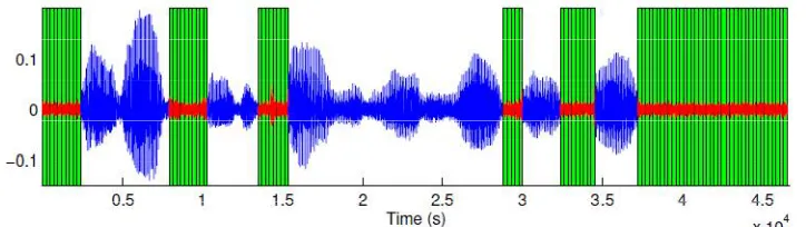
Fig. 6.1 Silence removal by VAD algorithm with white noise at 30 dB SNR
From the above figure, it is observed that the silence parts and speech segments are clearly distinguished with the advantage of the spectrum. At the SNR ratio 30dB, it is noted that the major portions of silence segments are easily separable. The unwanted segments can be eliminated with the concept of speech extraction. These parts are useful for the development of speaker data base.
Fig. 6.2 Silence removal by VAD algorithm with white noise at 20 dB SNR
The figure Fig.6.2 indicates the silence regions at the Signal to Noise Ratio of 20dB. Reasonable amount of speech segments are clearly available for the use of segmentation. The blue parts reflects the speech portion, where the noise pars are used for the elimination.
Fig. 6.3 Silence removal by VAD algorithm with white noise at 10 dB SNR
The effectiveness of the silence removal step on Speaker Recognition Rate is summarized in table 6.1 and 6.2.
Features Noisy speech 30 dB SNR
Noisy speech 20 dB SNR
Noisy speech 10 dB SNR MPCA with
silence removal step 96.02 94.3 93.25
PFA with
silence removal step 99.5 98.9 97.05
Table 6.1 Speaker Recognition Rate degraded by Additive Gaussian Noise
The results determined from the experiments after silence removal step show that the new feature vectors provide reasonable improvement over original features. Specifically, in presence of white noise at 30 dB SNR, the recognition rate is improved by 3.48 % with silence removal step by using PFA transform in place of MPCA transform.
Features Noisy speech 30 dB SNR
Noisy speech 20 dB SNR
Noisy speech 10 dB SNR MPCA with
silence removal step 96.5 95 90.25
PFA with
silence removal step 99.4 98.6 94.25
Table 6.2 Speaker Recognition Rate degraded by Additive channel Noise
Similarly in the presence of channel noise at 30 dB SNR, the improvement is 2.9 %. From the above results it is proved that in presence of more noise the performance of PFA transform is more effective than MPCA transform.
6.2.1 Population Vs Accuracy
In this experiment different population sizes of (150, 300, 450, 600, 750, 900, 1050, and 1200) are used. Recognition accuracy for a population size is computed by performing speaker recognition tests on S speakers randomly selected from 1500 speakers. Figures 6.4, 6.5 and 6.6 indicate the effect of population size on the speaker recognition rate under noisy conditions. The recognition accuracy with the application of PFA feature extraction is proved to be better than the original MPCA features.
Fig.6.4 Speaker Recognition rate as a function of number of candidates for additive white Gaussian noise and Channel noise at 10dB SNR : (a) without silence removal step (b) with silence removal step
90 92 94 96 98 100
150 300 450 600 750 900 1050
R
e
co
gn
it
io
n
A
cc
u
ra
cy
%
Population size
In order to investigate further the performance of the proposed PFA and FOLOS SVM algorithm method, the speaker recognition system is tested on noisy database prepared by using NIST database, channel noise and white Gaussian Noise. The experiment is conducted with 1200 speakers (712 males and 488 females) selected from the database. The model for every speaker is trained by clean speech of about 24 seconds containing 8 sentences.
Fig.6.5 Speaker Recognition rate as a function of number of candidates for additive white Gaussian noise and Channel noise at 20dB SNR : (a) without silence removal step (b) with silence removal step
The sentences contained with channel noise and white noises are used as two independent test segments. Testing has been conducted on the databases in two different sets, one with silence removal technique and another without it. The recognition accuracy is tested across three different SNRs using PFA-FOLOS combination.
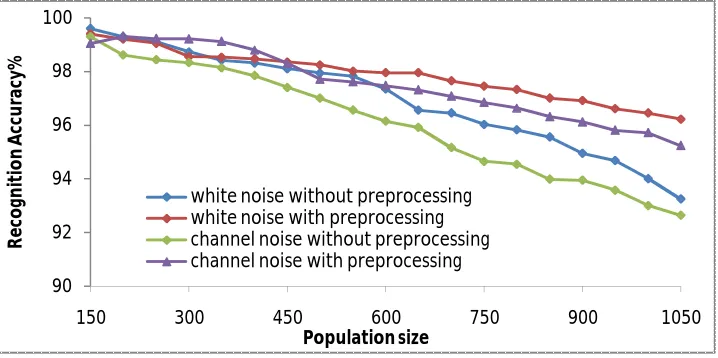
Fig.6.6 Speaker Recognition rate as a function of number of candidates for additive white Gaussian noise and Channel noise at 30dB SNR : (a) without silence removal step (b) with silence removal step
90 92 94 96 98 100
150 300 450 600 750 900 1050
R
e
co
gn
iti
o
n
A
cc
u
ra
cy
%
Population size white noise without preprocessing white noise with preprocessing channel noise without preprocessing channel noise with preprocessing
90 92 94 96 98 100
150 300 450 600 750 900 1050
R
ec
o
gn
it
io
n
A
cc
u
ra
cy%
Population size
From the results obtained from experiments, in presence of white noise of 30 dB SNR, the recognition rate is improved by 3.96 % (without silence removal step) and 4.28 % (with silence removal step) by using PFA transform and FOLOS SVM algorithm. Similarly in the presence of channel noise at 30 dB SNR, the improvement is 2.5 % and 2.55 % respectively. From the above results it is proved that in presence of noise the performance of the proposed system is more prominent.
VII. CONCLUSION
The results obtained from the experiments denote that the PFA transformation improves the speaker recognition rate as compared to the conventional features. Even with 50 % reduction in computational complexity, the PCA-FOLOS outscores the available state-of-art recognition techniques. The performance of the proposed method is always better as compared to MPCA in all situations. When compared with data base having different noise contents, the improvement is significant. As explained in above sections, although there is little bit of additional complexity in the training and testing phases, but that does not contribute to any significant increase in the delay when the overall response time of the recognition system is considered. In section V, the procedure for the candidate selection denoted by FOLOS is employed on the optimal set of feature vectors. The proposed technique is analytically proved and also empirically tested that the performance is better than existing recognition technologies in most of the cases due to its higher discriminating power. Also it is shown that the computational complexity of the classifier can be reduced significantly by taking relatively large number of speakers in the candidate selection process.
REFERENCES
[1] Homayoon Beigi, “Speaker Recognition: Advancements and Challenges”, Intech open access publisher, ISBN: 980-953-307-576-6, 2012. [2] D. A. Reynolds, “An Overview of Automatic Speaker Recognition Technology”, Proc. IEEE International Conference on Acoustics, Speech
and Signal Processing (ICASSP), pp. 4072-4075, 2002.
[3] J. J. Wolf, “Efficient acoustic parameters for speaker recognition”, Journal of the Acoustical Society of America, vol. 51, no.2, issue 6B, pp.2044–2055, 1972.
[4] Chan W. N., Zheng N, and Lee T, “Discrimination power of vocal source and vocal tract related features for speaker segmentations”, IEEE Transactions on Audio, Speech and Signal Processing, vol.15 no.6, pp.1884–1892, 2007.
[5] Murty K. S. R, Prasanna S. R. M, and Yegnanarayana B, “Speaker specific information from residual phase”, Int. conf. on signal processing. and comm. (SPCOM), IISc, Bangalore, pp.516 – 519, 2004.
[6] W. Hess, “Pitch Determination of Speech Signals”, IEEE Transactions on Neural Networks, vol.17, no.5,pp.1126-1140, 2006.
[7] Zhu Jian-wei, Sun Shui-fa, Liu Xiao-li and Lei Bang-jun, “Pitch in Speaker Recognition”, Ninth International Conference on Hybrid Intelligent Systems, vol.1, pp.33-36. 2009.
[8] Robert Rozman, Dusan M Kodek, “Using asymmetric windows in automatic speech recognition”, Journal of Elsevier, Speech Communication, vol.49, pp.268-276, 2007.
[9] Santiago D. Villalba, “Dimension Reduction”, Technical Report UCD-CSI-2007-7, University College Dublin, 2007.
[10] Philippe Reneveyy and Andrzej Drygajlo “Entropy Based Voice Activity Detection in Very Noisy Conditions”, Eurospeech proceedings, pp 1887-1890, 2001.
[11] Chunyan Liang, Lin Yang, Hongbin Suo, Junjie Wang, Yonghong Yan, “Factor analysis of Laplacian approach for speaker recognition”, International Conference on Acoustics, Speech and Signal Processing (ICASSP), pp.4221 – 4224, 2012.
[12] Peter Filzmoser, Karel Hron, Clemens Reimann and Robert Garrett, “Robust factor analysis for compositional data”, Journal of Computers and Geo-sciences, Vol.35, no.9, pp.1854-1861, 2009.
[13] Saeed K and Nammous M.K,“A Speech and Speaker Identification System: Feature Extraction, Description, and Classification of Speech-Signal Image”, IEEE Transactions on Industrial Electronics, vol.54, no.2, pp.887 –897, 2007.
[14] P.Rama Koteswara Rao, Dr. Y.Srinivasa Rao and D.Vijaya Kumar, “Principal Factor Analysis and SVM Based Effective Speaker Recognition” IEEE-Third International Conference on Computer Communication and Networking Technologies, 2012.
[15] C. J. C. Burges, “A tutorial on Support Vector Machines for pattern recognition”, Data Mining and Knowledge Discovery, vol.2, pp.121–167, 1998.
[16] W.Campbell, J.Campbell, T.Gleason, D.Reynolds and W.Shen, “Speaker verification using Support Vector Machines and high-level features”, IEEE Transactions on Audio, Speech, and Language Processing, vol.15, no.7, pp.2085–2094, 2007.
[17] John Duchi and Yoram Singer, “Efficient Online and Batch Learning Using Forward Backward Splitting”, Journal of Machine Learning Research, vol.10, pp.2899-2934, 2009.