Estimating Effective Population Size and Migration Rates From Genetic Samples Over Space and Time



Estimating Effective Population Size and Migration Rates From Genetic

Samples Over Space and Time

Jinliang Wang*

_{and Michael C. Whitlock}

*Institute of Zoology,Zoological Society of London, London NW1 4RY, United Kingdom and†_{Department of Zoology,}

University of British Columbia, Vancouver, British Columbia V6T 1Z4, Canada

Manuscript received July 24, 2002 Accepted for publication October 25, 2002

ABSTRACT

In the past, moment and likelihood methods have been developed to estimate the effective population size (Ne) on the basis of the observed changes of marker allele frequencies over time, and these have

been applied to a large variety of species and populations. Such methods invariably make the critical assumption of a single isolated population receiving no immigrants over the study interval. For most populations in the real world, however, migration is not negligible and can substantially bias estimates of

Neif it is not accounted for. Here we extend previous moment and maximum-likelihood methods to allow

the joint estimation ofNeand migration rate (m) using genetic samples over space and time. It is shown

that, compared to genetic drift acting alone, migration results in changes in allele frequency that are greater in the short term and smaller in the long term, leading to under- and overestimation of Ne,

respectively, if it is ignored. Extensive simulations are run to evaluate the newly developed moment and likelihood methods, which yield generally satisfactory estimates of bothNeandmfor populations with

widely different effective sizes and migration rates and patterns, given a reasonably large sample size and number of markers.

O

temporal data. This so-called “temporal approach” was ics theory has been in the estimation of genetic

and demographic properties of populations. Quantities pioneered by KrimbasandTsakas(1971), with

subse-quent substantial statistical refinements by others (e.g., such as the mutation rate, the migration rate, and the

recombination rate are all in principle estimable from PamiloandVarvio-Aho 1980;NeiandTajima 1981;

Pollak1983;TajimaandNei1984;Waples1989;

Wil-population genetic data, at least as products with the

effective population size. liamson and Slatkin 1999; Anderson et al. 2000;

Wang 2001a). These methods have been applied to a

The variance effective population size (Ne) is an

im-portant quantity in evolutionary biology, as a description large variety of species and populations (e.g., Funket

al. 1999;Labateet al. 1999;Fiumeraet al. 1999, 2000; of the rate at which genetic variance changes due to

genetic drift. A variety of methods have been developed Kantanenet al. 1999;Turneret al. 1999; see also many

earlier references cited in Williamson and Slatkin

to estimateNe(Schwartz et al. 1999), including

pre-1999). dictive equations based on life history data (reviewed

A key assumption made by all these approaches, how-inCaballero1994;WangandCaballero1999), the

ever, is that the only factor involved in allele frequency

lethal allelism approach (Dobzhansky and Wright

change is genetic drift. All systematic forces (selection,

1941), and a linkage disequilibrium approach (Hill

mutation, and migration) are assumed to be absent. In 1981). Several authors have developed methods to

esti-our view, it is often legitimate to ignore the effects of

mateNefor a population from temporal genetic data,

mutation on the timescale involved in most empirical that is, data on the frequencies of marker alleles taken

studies. It also may be reasonable to neglect the effects at two or more time points from the same populations.

of selection because direct selection on most markers In principle, if other population genetic processes such

may be unlikely to be strong enough to cause substantial as mutation, migration, and selection are negligible in

changes in their frequencies. (The effects of indirect their effects on allele frequency change over the time

selection acting on other linked loci on the allele fre-frame of the study, then the observed changes in allele

quency change of the marker locus may arguably be frequency can be assumed to be due to the effects of

included as a “drift” effect and legitimately included in genetic drift. Using what is known about the effects

aNe term.) However, for most populations the effects

of migration are not negligible. A major weakness of these temporal methods is that they ignore the effects

1_{Corresponding author:Institute of Zoology, Zoological Society of}

of migration, which can substantially bias estimates of

London, Regent’s Park, London NW1 4RY, United Kingdom.

E-mail: [email protected] Ne, either upward or downward (see below). The

pose of this article is to include the effects of migration requires about the demographic structure of the spe-cies. Other approaches include genetic stock identifica-in the estimation of demographic parameters from

tem-tion (Milner et al. 1985), assignment methods (

Ran-poral genetic data.

nalaandMountain1997), two-locus descent measures Migration can affect the estimation ofNein two ways.

(VitalisandCouvet2001), coalescent methods (

Niel-In the short term, migration can change allele

frequen-senandWakeley2001), isolation-by-distance methods cies quite quickly. Given that the temporal methods

(see review by Rousset 2001), and migration

matrix-estimate Neby measuring the pace at which allele

fre-likelihood models (BeerliandFelsenstein2001). The

quencies change, migration causes a population to

be-first two approaches require detailed knowledge about have as if strong drift was changing allele frequencies

the possible sources of migrants and do not allow for very rapidly, resulting in an estimate ofNethat is too low.

genetic drift. The latter four approaches assume that the In the longer term, the problem is reversed. Constant

populations are at an equilibrium between the effects of migration and drift would cause the populations to

ap-genetic drift and migration. There is a need for a method proach an equilibrium level of genetic differentiation

that does not make restrictive assumptions about ge-and the rate of change of allele frequencies in a deme

netic and demographic equilibria, yet allows simultane-to slow down simultane-to approach that predicted by the effective

ous estimation of the effects of drift and migration. size of the whole metapopulation. Thus the effective

Here we extend previous temporal methods for esti-population size of the deme would be substantially

over-mating the Ne of a single isolated population so that

estimated in the long term. These effects are discussed

they can be used to estimate Ne and m jointly for a

later in this article in more mathematical detail.

metapopulation. We first develop an expectation based This problem can be avoided by simultaneously

esti-on a moment estimatiesti-on approach, which allows an

matingNeand the migration rate, which is the approach

approximate description of the behavior of the estima-taken in this article. It turns out that while both

migra-tor and the system. We follow this by developing a likeli-tion and drift affect allele frequency changes in a

popu-hood method based on that ofWilliamsonand

Slat-lation, they do so differently in terms of the direction

kin(1999),Andersonet al. (2000), andWang(2001a).

and magnitude of these changes. Under migration, the

Extensive simulations are run to check the performance allele frequency of a focal population would tend to

of the moment and likelihood estimators in terms of become increasingly similar to that of the source

popula-precision and accuracy for the estimation ofNeandm.

tion. Under drift, however, the allele frequency of a

Two metapopulation models (a focal small population focal population changes purely at random, irrespective

receiving immigrants from an infinitely large source of that of the source population. Furthermore, the

mag-population and two small mag-populations connected by nitude of allele frequency change of a focal population

migration) are considered, and the applications of the depends on the allele frequency difference between the

methods to more complicated metapopulation models focal and source populations under migration.

Migra-(e.g., a small number of demes in island or

stepping-tion has no effect on alleles that happen to be at the

stone migration models) were checked by simulations. same frequencies both in the deme in question and in

As an example for the application of our methods, a the populations providing those migrants, but

migra-spatial and temporal genetic data set on Triturus newts tion is expected to change allele frequencies

substan-(Jehle et al. 2001) was reanalyzed by our methods for tially in cases when the source and recipient demes have

the simultaneous estimation of migration and drift. very different allele frequencies. Genetic drift, on the

other hand, is not affected by differences in allele fre-quencies among demes, but depends only on the local

DEFINITIONS AND ASSUMPTIONS

allele frequency. These differences in the patterns of

changes of allele frequencies due to migration and drift _{We use temporal data to estimate the effective size}

allow us to estimate them separately, so long as enough _{(Ne) and immigration rate (m) of a partially isolated}

data are from multiple loci. Fortunately, these kinds _{population. For brevity, we refer to the population for}

of data are often available with modern biochemical _{which parameters are being estimated as thefocal}

popu-methods. _{lation and that from which the migrants come as the}

The estimation of migration rate and migrant num- source population. Data and parameters for the source

ber has a long history. The oldest and most widely used population are given the subscriptA, and those for the

genetic method assumes that populations are at equilib- focal population,B. In the first section, we assume that

rium in a system approximated by Wright’s (1931) the source population is infinitely large and therefore

island model and then uses estimates of Wright’sFSTto not changing genetically through the time frame of the

calculate 1/(4Nem⫹1), wheremis the local immigra- study. In the section after that, we assume that both

tion rate (see Slatkin 1987). This method has been populations are finite and jointly estimate the properties

roundly criticized (Whitlock and McCauley 1999), of both. In the latter case, source and focal populations

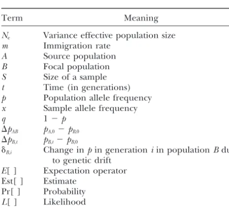
TABLE 1 loidy. For data from haploid species or loci, theNe

esti-mated by these models would be double the actual effec- _{Definitions of terms}

tive size.

For the infinite-source population model, a minimum _{Term Meaning}

of three samples is required to estimateNeandmof the

Ne Variance effective population size focal population: two temporally spaced ones from the

fo-m Immigration rate

cal population and one taken at any time from the _{A Source population}

source. For the two small population models, a mini- _{B Focal population}

mum of four samples is necessary, two temporally spaced S Size of a sample

t Time (in generations)

ones taken concurrently from each population. Let us

p Population allele frequency

denote the size of these samplesS, with subscriptsAor

x Sample allele frequency

B to describe whether the sample is from the source

q 1⫺p

or focal population, respectively, and a subscript t to

⌬pAB pA,0⫺pB,0

describe the generation in which the sample is taken. _⌬p

B,t pB,t⫺pB,0

ThusSB,0is the number of individuals sampled from the ␦_B,i Change inpin generationiin populationBdue

focal population in the initial generation. We usexto to genetic drift

E[ ] Expectation operator

refer to the relative frequency of a particular allele in

Est[ ] Estimate

a given sample. Thereforexis an estimator of the true

Pr[ ] Probability

frequency (p) of that allele at that time in that

popula-L[ ] Likelihood

tion. For convenience, we defineq⫽1⫺ p. These quanti-ties,x,p, andq, are subscripted in the same way asS.

Several summary statistics of these quantities turn out

these conditions, and assuming that migration precedes to be useful. We define⌬pAB⬅pA,0⫺pB,0to be the initial

population regulation, the allele frequency at genera-difference between the allele frequencies of the two

tioniis given by populations and ⌬pB,t ⬅ pB,t ⫺ pB,0 to be the change

in allele frequency by generation t in deme B. In the

pB,i⫽(1 ⫺m)pB,i⫺1⫹ mpA⫹ ␦B,i. (1)

derivations of the moment-based estimators, we also use

␦B,ito refer to the change in generationidue to genetic Note then that

drift of the allele frequency in population B. Each of

pB,1⫽pB,0 ⫹m⌬pAB⫹ ␦B,1. (2) the quantities can refer to populationAif the subscript

Bis replaced by A. _{Expanding across generations, we can find}

We make several assumptions throughout. These are

that the alleles under study are not under direct selec- _{pB,t⫽pB,0 ⫹m⌬pAB}

兺

t⫺1

i⫽0

(1⫺ m)i⫹

兺

t

i⫽1

␦B,i(1 ⫺m)t⫺i, (3)

tion, that mutation is a negligible source of allele

fre-quency change, that potential sources of migrants to _so

the focal populations can be identifieda priori, that all

⌬pB,t⬅pB,t⫺pB,0⫽ ⌬pAB(1⫺(1⫺m)t)⫹

兺

t

i⫽1

␦B,i(1⫺m)t⫺i. (4)

samples are randomly taken from their populations, and that the sampling event does not change the

avail-able pool of reproductive individuals. The latter can be Under the assumptions of Wright-Fisher sampling, the

␦terms are independently binomially distributed. The

realized by sampling after reproduction, sampling with

replacement, or sampling from a population much expected value of all of the␦terms is zero, because drift

does not change on average the allele frequency. The larger than the sample. This sampling scheme therefore

corresponds toWaples’s (1989) plan 1. variance of each of these terms is given bypB,i(1⫺pB,i)/

Nefor haploids orpB,i(1⫺pB,i)/2Nefor diploids. In real-Table 1 summarizes most of the terms used in this

article. ity, we do not know pB,i for any generation between

samples, and we can only estimatepB,i for generations

in which there was a sample. This uncertainty is the

IMMIGRATION FROM AN INFINITE-SOURCE _{root of error in the estimation of statistics derived from} POPULATION

these equations. In this article, we first estimate this error by using the approximate moments of the

distribu-Theoretical background:Imagine that the focal

popu-lation is receiving migrants at rate m per generation tion of allele frequencies, and then we describe a

likeli-hood approach to the estimation ofNeandm.

from an infinite, unchanging source population. For

effectively neutral alleles, changes in allele frequency Moment approximations:Neandmaffect the first and

second moments of the change in allele frequency over over a short period of time are a function of the local

effective population size and migration rate. Mutations time. Under certain circumstances, we can use these

moments to estimatemandNe. We do this in a two-step

are negligible compared to drift and migration because

allele frequencies at all loci and then using this value

mˆ ⫽ 1⫺ t

冪

冢

W

冣

兺

L

l⫽1

wlFl, (8)

in the estimation of Ne from the second moment of

allele frequency change.

Estimating the migration rate:The change in allele fre-quency is given by Equation 4 above. Taking the

expecta-where the weight for locusliswl⫽(⌬xAB)2,Fl⫽ ⌬xB,t/

tion of⌬pB,twe find _⌬

xAB, andWis the sum ofwl across loci.

Estimating Ne: Under the assumption that the total

E[⌬pB,t]⫽ E[⌬pAB](1⫺(1⫺ m)t) , (5)

change in allele frequency per generation is not large

because the expected values of all the␦terms are zero. _{(i.e.,Neis not very small andmis not very large), each}

Assuming thattis known without error, we can therefore _{of the terms in the equation describing allele frequency}

make a one-locus estimate of (1⫺(1⫺m)t_{) from}⌬_p

B,t/ change is roughly independent of the others. The

vari-⌬pAB. ance in allele frequency change at generationidue to

To predict the optimal sampling strategy and to ap- _{genetic drift within the focal population is V[␦B,i] ⫽}

proximate standard errors, we estimate the error vari- _{pB,iqB,i/2Ne,B. If the allele frequency is not changing}

rap-ance of an estimate ofm. The expected error in estimat- _{idly, then we can assume that the value ofpqis}

approxi-ing a ratio is an approximate function of the error _{mately the same each generation. A reasonable}

estima-variance of estimating the numerator and the denomi- _{tor of the mean value ofpqispq⬇(xB,0(1⫺xB,0)⫹xB,t}

nator and the error covariance between the two (see _{(1⫺xB,t))/2. This is implicitly assuming that the allele}

Lynch and Walsh 1998, Appendix 1). The error in _{frequency on average takes a linear path from the initial}

estimating (1⫺ (1 ⫺m)t_{) can be approximated from}

to the final value, but in any case is anad hoc

approxima-the error in estimating⌬pB,t/⌬pAB. The error variances tion. Then using Equation 4, we can find

(Verr[ ]) and error covariance (COVerr) are given by

E[⌬pB,t2]⫽ ⌬pAB2(1 ⫺(1⫺ m)t)2⫹M

冢

pq

2Ne,B

冣

, (9)

Verr[⌬pB,t]⬵

pB,0qB,0 2SB,0

⫹pB,tqB,t

2SB,t

,

where M ⫽ (1 ⫺ (1 ⫺m)2t_)/((2 ⫺

m)m). Again, the coefficient of Ne,Bof 2 drops out when this formula is

Verr[⌬pAB]⫽

pA,0qA,0 2SA,0

⫹pB,0qB,0 2SB,0

,

used for haploids. From Equation 9 and using the esti-mate ofm, we obtain an estimator of 1/(2Ne,B),

COVerr[⌬pB,t,⌬pAB]⫽

pB,0qB,0 2SB,0

. (6)

Est

冤

冥

⫽ E[⌬pB,t2]⫺ ⌬pAB2(1⫺(1 ⫺mˆ)t)2

Mˆ pq , (10)

Note that the 2’s in the denominators drop out when

whereMˆ _⫽ (1⫺(1 ⫺mˆ)2t_)/((2⫺_m

ˆ)mˆ). these equations are applied to haploids. The

approxima-In general we do not have exact information about tion in the first equation here comes from using the

the change in population allele frequencies, but only

initial value ofpqto predict the amount of variance in

an estimate based on sample data. Because of sampling final allele frequency due to genetic drift.

variance, E[⌬xB,t2] is biased upward as an estimator of

Using these last equations and Equation A1.19b from

⌬pB,t2:

Lynch and Walsh(1998), we can find the expected error variance for the estimate of (1⫺(1 ⫺m))t_:

E[⌬xB,t2]⫽ ⌬pB,t2⫹

pB,0qB,0 2SB,0

⫹pB,tqB,t

2SB,t

. (11)

Verr[1⫺(1⫺mˆ)t]⬵

冢

1 ⌬pAB冣

2

Thus we can estimate

⫻

冢

冢

(1⫺m)2t 2SB,0

⫹ 1 2SB,t冣

⫹pA,0qA,0

冢

(1⫺(1⫺m)t₎2

2SA,0

冣冣

.

Est

冤

冥

⫽

冤

冢

xB,0(1⫺ xB,0) 2SB,0

⫹xB,t(1⫺xB,t)

2SB,t

冣

(7)

If the three sample sizes are roughly equivalent, then _{⫺ ⌬}

xAB2(1 ⫺(1⫺ mˆ)t)2

冥

the error in estimating m is influenced more by the

allele frequency in population B than by that in the

source population, especially if the productmtis small. The error variance per locus for estimating 1/(2Ne) is

The terms involving only the sample sizes,m, andtare approximately proportional to 1/pq (calculations not

presumably constant across loci, so the error variance shown), so a minimum-variance estimator of 1/(2Ne)

is largely proportional to 1/(⌬pAB)2. The minimum vari- can be obtained by weighting alleles by pq

approxi-ance possible when combiningL loci can be obtained mately, estimated by (xB,0(1 ⫺xB,0)⫹xB,t(1 ⫺xB,t))/2.

by weighting each locus by the inverse of its expected Choosing the right value of t:With a large separation in

error variance. The best estimator ofmis given approxi- time between the first and second samples, estimates of

mbecome problematic. The estimate of (1⫺(1⫺m)t₎

becomes more and more similar for different values of

mastgets larger (limt→∞[␦(1⫺(1⫺m)t)/␦m]⫽0), yet

the error variance in estimating this quantity increases linearly with t. Furthermore, as t increases, the allele frequency change approaches a distribution deter-mined largely by the relative sizes of the effective size

and m, rather than by the absolute values of either.

Whent is large enough that the populations reach an

equilibrium between genetic drift and migration, then

mˆ → 0, irrespective of the actual true migration rate.

This is clear by inspecting the single-locus estimator ofm,

mˆ ⫽1⫺

√

increases and⌬xB,t/⌬xABis expected to reach a constant

smaller than one with time, therefore resulting inmˆ →0. If the time interval is too short andmtoo small, then

there is less power to measurembecause too few

migra-tion events may have occurred. Larger samples with more informative markers are therefore necessary to

obtain a good estimate ofmwhen (1⫺ m)t

is close to one or zero.

Similarly, the estimation of Ne is also biased if the

sampling interval is too long. Ast→∞, we havemˆ →0

shown above and Equation 10 reduces to Est(1/2Ne,B)⫽

E[⌬p2

B,t]/(t pq). If the source population is infinite in

size, then E[⌬p2

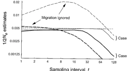
B,t] tends to a constant as t → ∞, and Figure1.—Means (A) and coefficients of variation (B) of

estimates of 1/(2Ne) andmas a function of sampling interval thereforeNˆe,B→∞. If the source population has a finite

t(in generations). The population contains 11 subpopulations

size, then E[⌬p2

B,t] continues to increase as t → ∞(so

of an equal Ne (100), migrating in the island model with long as the alleles are not fixed in the population), but

rate 0.2. After the population reaches quasi-equilibrium, two

at a slower rate corresponding to the total size of the _{samples separated bytgenerations are taken from each of}

focal and source populations. In both cases, the estimate the 11 subpopulations. The size of each sample from the focal

subpopulation is 200 individuals, and the sample from any

ofNe,Bapproaches the effective size of the whole species

source subpopulation is 10 individuals. The 20 samples from

rather than that of the focal population. Again, there

the source subpopulations are combined into a single sample.

is less power for estimatingNe,BiftandS/(Ne,B) are too

For each sample, 20 loci, each having four alleles, are

geno-small. With a small quantity oftS/(Ne,B), the change in _{typed and used in the estimation. In the top graph, the}

aver-allele frequency due to drift would be overwhelmed by ages over 10,000 replicate estimates ofmand 1/(2Ne) from

the moment estimator are denoted by thin and thick solid

that from sampling.

lines, respectively. The true value for mis denoted by the

As a numerical example, Figure 1A shows the average

horizontal thin dashed line, and the true values of 1/(2Ne) estimates of 1/(2Ne,B) andmover 10,000 replicates plot- _{for the focal subpopulation (0.005) and the whole population}

ted against sampling intervalt, and Figure 1B shows the _{(1/2224) are denoted by the top and bottom horizontal thick}

coefficients of variation (CV) of the estimates whent⫽ dashed lines. Both axes of this graph are in log scale. In

the bottom graph, the coefficients of variation over 10,000

1–12 where the estimation is unbiased. (Methods for

estimates ofm and 1/(2Ne) are denoted by thin and thick

these simulations are given in theappendix.) The true

lines, respectively, from the moment estimator.

values being estimated are 1/(2Ne,B)⫽0.005 (Ne,B⫽100)

andm⫽0.2 for the focal population, which is assumed

to be in a metapopulation containing 10 other

popula-m, the effective sizes of the focal and source populations, tions of the same size (Ne⫽100) with an island

migra-and the initial genetic differentiation when the first tion model. The effective size of the source population

sample was taken (see below). is thereforeⵑ1000, sufficiently large although not

infi-For this specific numerical example, the estimation is nite. As can be seen, estimates of both 1/(2Ne,B) andm

unbiased whenⵑt⬍12. The precision of the estimators

are close to the true values whentis small, but approach

changes considerably over this short sampling period

the true values for the whole species, 0.00045 (Ne ⫽

(Figure 1B). As expected, the best estimates are ob-1112, calculated using the known parameters) and 0,

tained at an intermediate value oft (t ⫽ 2–4 for the

with increasingt. The maximum number of generations

example). The optimal sampling interval depends, allowed for valid joint estimates of 1/(2Ne,B) andmand

again, onm, the effective size of the focal population

the number of generations required to reach the

sample was taken. With decreasingmand/or increasing initial differentiation, for example, the optimaltis ex-pected to increase.

In experimental design, it is difficult to determine beforehand the optimal interval between sampling for maximum power of the temporal method, because the power depends partially on the parameter being

esti-mated (seee.g., Equation 7). Without any prior

knowl-edge of the demographic history of the populations in question, it is reasonable to consider a short rather than a long sampling interval. While a too long sampling interval results in biased estimates ofNe andm, a too

Figure2.—Bias of 1/(2Ne) estimates as a function of

sam-short sampling interval only decreases the precision of

pling interval (in generations). The true value being estimated

the estimates. With powerful statistical methods (e.g.,

is 1/(2Ne) ⫽ 0.005 (Ne ⫽ 100) denoted by the horizontal

maximum likelihood shown below) and large sample _{dashed line, and the true migration rate is 0.1. The}

popula-size and marker information, the estimation precision _{tions are assumed to have no previous migration (case A) or}

can be improved greatly even if t is as short as one be at drift-migration equilibrium (case B) when the first

sam-ple from the focal population is taken. For cases A and B, the

generation.

averages over 1000 replicate estimates of 1/(2Ne) are denoted

The consequences of assuming that m⫽0:Other methods

by thin and thick solid lines, respectively, from the moment

using temporal data for estimating the effective size _{estimator developed herein that takes immigration into}

ac-have assumed that the immigration rate is zero. We can count, by thin and thick dashed lines, respectively, from the

moment estimator ignoring immigration (Equation 13). In

use the equations above to investigate the effects of

the estimation, we assumed 20 loci, each having four alleles,

making this assumption when it is in fact false.

and two samples from the focal and one sample from the

Whenm→0, the expected change in allele frequency

source population, each sample having 200 individuals. Note

is zero,M ⫽t, and Equation 12 reduces to _{that both axes are in log scale.}

Est

冤

冥

⬵⌬xB,t2⫺(xB,0xB,0/(2SB,0)⫹xB,txB,t/(2SB,t))

tpq , (13) focal population, no matter whether the assumption of

m⫽ 0 is made or not. These biases can be indefinitely

which is similar toNei andTajima’s (1981) estimator _large.

usingFc. _{Figure 2 shows the biases of N}

e estimation when a

Whenm⬎0, the variance in allele frequency change _{false assumption ofm⫽0 is made. The true parameter}

over the interval between samples is a function of both _{values areN}

e⫽100 andm⫽0.1, and the populations

genetic drift and migration. This can be either greater _{are assumed to be either completely differentiated (no}

or smaller than that expected by drift alone, depending _{previous migration, case A) or at drift-migration}

equilib-on, among other parameters,t. In the short term, the _{rium (case B, whereF}

st⬇0.02) when the initial sample

change in allele frequency due to the joint effects of _{is taken. Ignoring migration results in an overestimation}

migration and drift will be larger than that expected by _{of 1/(2Ne) when sampling interval (t) is small and}

un-drift alone. If t ⫽ 1, for example, we have E[(pB,t ⫺ _{derestimation when tis large. Compared with case A,}

pB,0)2]⫽ ⌬pAB2m2⫹pB,0(1⫺pB,0)/2Ne,B. In this case, there- _{the initial overestimation of 1/(2Ne) in case B from}

fore, the squared change in allele frequency is increased _{ignoring migration is much smaller, because the}

popula-relative to that due to drift only, which ispB,0(1⫺pB,0)/ _{tions are more similar genetically (}⌬_{pABsmall) and}

there-2Ne,B. Falsely assuming that m ⫽ 0 would on average _{fore migrants have less effect on allele frequency changes.}

cause an overestimate of the amount of drift and an _{With a largermand smallerNe, the initial overestimation}

underestimate ofNe,B. In contrast, as the time between of 1/(2_Ne) can be dramatic even when the populations

samples gets large, the change in allele frequency is _{are initially at equilibrium (data not shown). For both}

constrained by migration to a term only somewhat larger _{cases, the estimation is reasonably good for a large range}

than the squared initial difference in allele frequency of sampling interval when immigration is accounted for.

between the source and focal populations: limt→∞E[(pB,t⫺ However, the sampling interval cannot be too long.

pB,0)2] ⫽ ⌬pAB2 ⫹ pB,0(1 ⫺ pB,0)/(Ne,Bm(2 ⫺ m)). With Otherwise, 1/(2Ne) is increasingly underestimated with

an increasing sampling interval (t), therefore, a false t, approaching the true value for the whole species.

assumption ofm⫽ 0 would cause a downward bias in Likelihood model:Let us first consider a single locus

the estimation of the amount of genetic drift and an with two alleles, and we focus on a particular allele. For

upward bias in estimatingNe. As the number of genera- brevity in this subsection, subscriptBis dropped for the

tions between samples continues to get larger, however, focal population. To estimate m and Ne of the focal

the estimate would approach the effective size of the population jointly, at least two temporally spaced

population (A) are necessary. Because the three sam- wherep*j ⫽ (j/2Ne)(1⫺m)⫹ mpAand (i,j⫽ 0, . . . ,

pling events are independent, the probability of getting 2Ne). This accounts for the deterministic change in

al-a set of sal-amples with al-allele frequencies denoted byxis lele frequency due to migration as well as the genetic

sampling due to drift. Given the initial distribution of Pr[x0,xt,xA|p0,pt,pA]⫽Pr[x0|p0]Pr[xt|pt]Pr[xA|pA]. (14)

allele frequency of the focal populationP0[a column

Each of these samples can be assumed to follow a bino- vector of 2Ne⫹1 elements with values 1/(2Ne⫹1) or

mial distribution (seeWaples1989 for a discussion of 1/(2Ne⫺1) as assumed above] and values ofpA,Ne, and

when this is appropriate); therefore m, the distribution aftertgenerations,Pt, is calculated by

the recurrence equation Pr[x|p]⫽

冢

2Sx

冣

2Sx₍₁⫺ _p)2S(1⫺x)_,

Pt⫽TtP0. (17)

whereSis the number of diploid individuals sampled. _{These are all the parts necessary to calculate the}

likeli-For haploid species, the coefficient 2 of S should be _{hood, above. For multiple independent, biallelic loci,}

dropped. _{the joint likelihood of N}

e and m is calculated as the

The likelihood (L) of a particular set of values ofNe _{product of the likelihoods for each locus.}

and m is the probability of observing the data given _{For loci with more than two alleles, the calculation}

those values. We have, therefore, _{of the likelihood function is problematic. The number}

of possible configurations,C ⫽ (2Ne ⫹ k⫺ 1)!/(2Ne!

L[Ne,m|x0,xt,xA]⫽Pr[x0,xt,xA|Ne,m]

(k⫺1)!) for a diploid locus withkalleles (Feller1950;

⫽

_兺

p₀,pt,pA

Pr[x0,xt,xA|p0,pt,pA]Pr[p0,pt,pA|Ne,m].

WilliamsonandSlatkin1999), increases rapidly with

k, prohibiting the evaluation of the exact likelihood due (15)

to the limitations of computer memory and processing

As we can see, the key problem for the likelihood func- _{speed. For a moderate value ofN}

e, evenk⫽3 poses a

tion is to calculate Pr[p0,pt,pA|Ne,m]. By the definition _{serious computational problem for the likelihood}

of conditional probability, we have

method. Anderson et al. (2000) proposed a Monte

Carlo method to evaluate the likelihood function with Pr[p0,pt,pA|Ne,m]⫽Pr[pt|p0,pA,Ne,m]Pr[p0,pA|Ne,m]. (16)

data on multiallelic markers. Their method does not

Determining the second term in Equation 16, Pr[p0,

need much storage but is highly demanding

computa-pA|Ne,m], is potentially quite tricky. If we assume,

how-tionally and may not converge whenkis large (say,k⫽

ever, that we do not know anything about how close the

10) or some alleles are not observed in all samples. To focal population is to a migration-drift equilibrium nor

simplify the likelihood computation for multiallelic loci, about the history of these populations, then this can be

we follow our previous approach (Wang2001a), which

given reasonably as a product of the uniform

distribu-transforms a k-allele locus into k biallelic “loci,” each tions ofp0andpA, Pr[p0,pA|Ne,m]⫽Pr[p0|Ne]⫻Pr[pA].

having one of the k alleles with all the other alleles

As Williamson and Slatkin (1999) point out, the

pooled. The overall log-likelihood is approximated by range of the possible values for the uniform prior,

the sum of the log-likelihoods across loci multiplied by

Pr[p0|Ne], will depend on whether only alleles

segregat-the factor of (k⫺1)/kto account for the dependence

ing in the initial population are used. There are 2Ne⫹

among such converted loci. 1 possible configurations for a biallelic locus in a

popula-The likelihood method can also use more than two tion with sizeNe, of which 2Ne⫺1 are polymorphic. With

samples from the focal population simultaneously to the uniform prior, therefore, any possible configuration

obtain a meanNe and an averagemduring the whole

for the starting frequencyp0has an equal probability of

sampling period. If samples are taken from the focal either 1/(2Ne⫹1) or 1/(2Ne⫺1) if we consider all or

population at generationst0,t1,t2, . . . ,tg, then the only polymorphic configurations, respectively. For the

joint likelihood ofNeandmis source population, we use a discrete approximation,

Pr[pA,j ⫽ j/J] ⫽ 1/(J ⫹ 1) for j ⫽ 0, 1, 2, . . . , J.

L[Ne,m|xt0,xt1,xt2, . . . ,xtg,xA]⫽ 兺 p_t0,p_t1,p_t2,...,p_tg,p_A

The estimation does not change essentially once J is

reasonably large (say, 1000), as expected.

⫻Pr[xt0,xt1,xt2, . . . ,xtg,xA|pt0,pt1,pt2, . . . ,ptg,pA]

The first term in Equation 16, Pr[pt|p0,pA,Ne,m], can

be calculated by using the transition matrixT(Ewens

⫻Pr[p0,pA|Ne,m]兿

i⫽1,g

Pr[pti|pt(i⫺1),pA,Ne,m] . (18)

1979). The probability of a transition from thejth

con-figuration of the parental population at timet ⫺1 to

Similarly, a continuous growth model, such as exponen-theith configuration of the offspring population at time

tial growth, could be fitted to the temporal data and

tis

joint estimates of initial effective size, growth rate, and

immigration rate can be obtained (Wang 2001a). A

Tij⫽

冢

2Ne

i

冣

i₍₁⫺

p*j )2Ne⫺i,

rate over the sampling period could be developed using For the case oft⬎1, moment estimators for bothm

andNebecome much more complicated (especially the

multiple samples.

latter) and are not shown here.

Likelihood estimator:The likelihood of the effective

TWO FINITE DEMES _{sizes (N}

e,A,Ne,B) and immigration rates (mA,mB) of demes

AandBgiven the temporal data (xA,0,xA,t,xB,0,xB,t) is

Up to this point, we have considered the demographic

properties of a single deme that receives immigrants _L[N

e,A,mA,Ne,B,mB|xA,0,xA,t,xB,0,xB,t]⫽ 兺 p_A,0,p_A,t,p_B,0p_B,t

from an effectively infinite source, that is, a source so large that over the time course of the study it is not

⫻Pr[xA,0|pA,0]Pr[xA,t|pA,t]Pr[xB,0|pB,0]Pr[xB,t|pB,t]

changing appreciably in allele frequency. While this is likely to be a reasonable approximation in many cases,

⫻Pr[pA,0|Ne,A]Pr[pA,t|pA,0,Ne,A,mA,Ne,B,mB]

there are examples in nature where only a few relatively

small demes serve as the only source of migrants to each _⫻Pr[p

B,0|Ne,B]Pr[pB,t|pB,0,Ne,A,mA,Ne,B,mB] . (22)

other. This case is more difficult, both analytically and

In Equation 22, each of the four samples follows a bino-computationally, but here we consider the case of two

mial distribution for Pr[x|p], the initial allele frequency small demes as a beginning to such an analysis.

of each population is assumed to be in a uniform distri-The allele frequency at a neutral locus will change

bution, and the allele frequency distribution of each over a single generation in the two populations

ac-population at generation t can be calculated by using

cording to

the transition matrix.

PA,i⫽(1⫺ mA)pA,i⫺1⫹mApB,i⫺1⫹ ␦A,i In principle, the exact likelihood could be worked

out for any set of the four parameter values, but in

pB,i⫽(1⫺ mB)pB,i⫺1⫹ mBpA,i⫺1⫹ ␦B,i. (19)

practice this would be computationally intensive for

any-Moment estimator:We can find a moment estimator _{thing but small population sizes and small sampling}

for the two migration rates for this two-finite-deme case, _{interval (t). The total number of configuration}

combi-if we consider the change in the dcombi-ifference in allele _{nations that need to be considered in Equation 22 is}

frequency between the demes over time. We consider _{((2Ne,A ⫹ 1) (2Ne,B ⫹ 1))}t _{for a biallelic locus, which}

the simple case in which the samples are separated by _{increases exponentially with sampling intervalt.}

There-only a single generation, and so we drop the subscript _{fore, we use the transition matrix method for the exact}

notation for time. Taking the expectations of Equation _{calculation of the likelihood for samples separated by}

19 above and remembering that the expected values of _{only a single generation (t⫽1) and use a Monte Carlo}

␦Aand␦Bare zero, we find approach to approximate the likelihood for samples

witht ⬎1.

mˆA ⫽ ⌬

pA

⌬pAB

, Equation 22 could easily be extended to more than

two samples from each deme with little increase in com-putational demands. It could also be extended to more

mˆB⫽ ⌬

pB

⌬pAB

. (20) _{than two demes, but the computational intensity}

in-creases prohibitively with the number of demes, because

The error variance in estimating migration rates would _{of the exponential increases in configuration}

combina-be proportional to 1/⌬p2

AB, so we can find a low variance _{tions and the number of parameters for joint estimation.}

estimator of the migration rates by weighting informa-tion from each allele by⌬p2

AB.

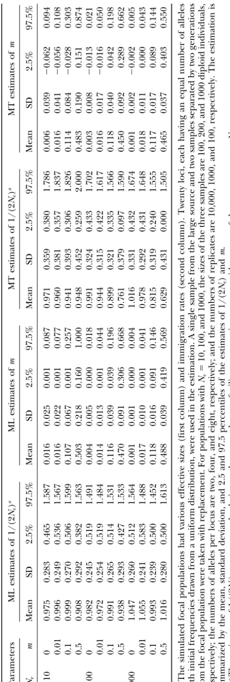
SIMULATION RESULTS

Finding an estimator of the effective size of each deme

is also possible. The variance of the change in allele _{Infinite source: Methods for these simulations are}

frequency over time due to drift for populationAis _{summarized in theappendix. For focal populations with}

wide ranges of effective size and immigration rates, the

V[␦A]⫽E[␦2A]⫽

p⬘A(1⫺p⬘A)

2Ne,A

, (21) _{maximum-likelihood and moment estimates of 1/(2Ne)}

andmfrom simulations are summarized in Table 2. The

sample sizes used in the simulations are large, but not where p⬘A is the expected allele frequency after

migra-tion, which can be estimated from Equation 19 by setting unrealistic. Indeed, a large sample size is important for

the temporal methods; otherwise, the apparent changes

␦A ⫽ 0 and using the estimated migration rates and

initial allele frequencies. Thus the effective size can be in allele frequency would be dominated by sampling

error rather than by genetic drift. For most natural estimated in this case in a manner similar to the Waples

technique, except instead of using the initial allele fre- populations, the actual census population sizes could

be orders of magnitude larger than the effective sizes quency, one uses the expected initial frequency after

migration. Similar derivations for Ne,B can also be ob- (Frankham1995), making both large samples and

Figure4.—Log likelihood as a function of estimates ofNe

andmfor a particular simulated data set with true parameter valuesNe⫽100 andm⫽0.1. A single sample from the large

source and two samples separated by two generations from the focal population were taken with replacement, the sizes of the three samples being 200 diploid individuals. Twenty loci, each having four alleles, were used in the estimation.

precision. In contrast to 1/(2Ne), both the moment and

the maximum-likelihood methods give similar estimates

ofm. However, some moment estimates ofmare

nega-Figure 3.—The frequency distributions ofNe(A) and m _{tive whenmis small.}

(B) estimates from maximum-likelihood (thick lines) and

mo-In general, both maximum-likelihood and moment

ment (thin lines) estimators over 10,000 replicates. Two

sam-methods give reasonable estimates of Ne and m. The

ples separated by four generations are taken from the focal

population, and one sample is taken from the infinite-source accuracy and precision of the two estimators are similar

population. Each sample contains 100 diploid individuals, _{form, but the likelihood method is better forNe. This} which are genotyped for 10 loci, each having four alleles. The _{is partially because moment methods must use the} esti-true parameter values areNe⫽100,m⫽0.1, indicated by the

mate ofmin estimatingNe. Such a two-step estimation

dashed vertical lines.

procedure is expected to be inferior to the joint

estima-tion ofmandNefrom the likelihood approach, because

the estimation error ofmis not accounted for in estimat-The maximum-likelihood estimator gives unbiased

es-timates of 1/(2Ne) in all cases considered. The coeffi- ingNe. Also, whenmis large and therefore the changes

of allele frequencies are rapid, the approximation to cient of variation of the estimates is roughly one-quarter,

with 95% of the estimates being in the range of ⵑ50 the mean value ofpqin deriving the moment estimator

ofNemay be no longer good enough.

and 150% of the true values. The moment estimator

underestimates 1/(2Ne) slightly when m is large and The distribution of the estimates ofNe[or 1/(2Ne)]

generally has a long tail, with a significant proportion sample size is small relative toNe. Increasing sample size

can decrease the bias dramatically. For the case ofNe⫽ of the estimates being much larger (smaller) than the

true value. This is similar to the observation made on

100 andm⫽0.5 in Table 2, for example, the mean⫾

SD of the moment estimates of 1/(2Ne) improves to the case of a single isolated population (NeiandTajima

1981; Waples 1989; Wang2001a). For the particular

0.9⫾ 0.3 (relative to the true value) when the sample

size is 500 individuals. The estimates from the moment parameter set ofNe⫽ 100, m ⫽ 0.1, the distributions

ofNeandmestimates over 10,000 replicates are shown

estimator are generally more dispersed than those from

the maximum-likelihood estimator. in Figure 3. Again, there is very little difference in the

distribution of estimates of m between the two

tech-The maximum-likelihood method overestimates m

slightly only when mis small in very small populations niques, the mean⫾ SD being 0.114⫾0.048 for

maxi-mum likelihood and 0.115 ⫾ 0.049 for the moment

(Ne ⫽ 10). This is expected because

maximum-likeli-hood estimates have a lower bound at zero. Increasing estimator. ForNeestimation, however, maximum

likeli-hood is much more accurate and precise than the mo-sample size or marker information (number of loci and

TABLE 3

Maximum-likelihood and moment estimates of 1/(2Ne) andmrelative to their true values, using different numbers of samples

Relative estimates of 1/(2Ne) Relative estimates ofm

No. of

samples Mean SD 2.5% 97.5% Mean SD 2.5% 97.5%

The maximum-likelihood estimator

2 1.013 0.286 0.508 1.620 1.078 0.456 0.229 2.065

3 1.005 0.190 0.638 1.393 1.082 0.299 0.568 1.723

4 1.013 0.156 0.712 1.336 1.048 0.246 0.620 1.569

5 1.020 0.134 0.785 1.283 1.026 0.222 0.647 1.505

6 1.014 0.123 0.782 1.260 1.020 0.195 0.701 1.435

The moment estimator

2 0.748 0.415 0.016 1.616 1.179 0.341 0.565 1.857

3 0.722 0.307 0.174 1.363 1.179 0.250 0.750 1.688

4 0.728 0.243 0.264 1.240 1.174 0.221 0.775 1.618

5 0.737 0.222 0.342 1.214 1.171 0.207 0.815 1.628

6 0.734 0.194 0.401 1.152 1.179 0.180 0.873 1.577

The estimates of 1/(2Ne) andm, relative to the true parameter values 1/(2Ne) ⫽0.01 and m⫽0.2, are

obtained from the maximum-likelihood and moment estimators using a single sample from the source and different numbers of samples taken from the focal population every two generations. The size of each sample is 50 individuals, and 10 loci, each having 10 alleles, are used in the estimation.

is 0.0049⫾0.0020 for maximum likelihood and 0.0041⫾ sample sizes, which lead to a high proportion of rare

alleles in the samples (Wang2001a).

0.0025 for the moment estimator. The latter gives a

significant proportion of extremely largeNeestimates. Quasi-infinite source, the island model and the

step-ping-stone model: In reality, the source population is

Typically, the likelihood surface is smooth and has

a single maximum. This means that a single arbitrary not infinite in size, although it could be very large.

Moreover, there can be different numbers of source starting point is sufficient to obtain

maximum-likeli-hood estimates using Powell’s quadratic convergence populations for a focal population with migration in

different patterns. As long as we can identify the source method (Presset al.1996). Of course the starting point

affects the time spent in the search process, and the populations a priori, however, the parameters for the

focal population can be estimated approximately using values provided by the moment estimates usually act as a

good starting point close to the point with the maximum the methods developed for the infinite-source model

by treating the source populations collectively as the likelihood. For a particular replicate withNe⫽100 and

m⫽ 0.1 in Table 2, the likelihood curve is shown in single “infinite” source. Here we explore numerical

ex-amples to show that the infinite-source model is very

Figure 4. The maximum-likelihood estimates ofNeand

mare 102 and 0.107, respectively, with 95% confidence robust and works well for small source populations with

various models of migration. intervals being 65–172 and 0.038–0.191, respectively.

Multiple samples over time can increase the estima- Consider a metapopulation consisting of 21

popula-tions of equal effective sizeNe. Each population receives,

tion precision for the average 1/(2Ne) and m during

the entire sampling period. Table 3 summarizes the at each generation, a proportion ofmmigrants taken

equally from each of the remaining 20 populations in estimates of 1/(2Ne) andm, relative to the true

parame-ter values of 1/(2Ne)⫽ 0.01 andm⫽ 0.2, from maxi- the island model or from each of the two neighboring

populations in the circular stepping-stone model. For mum-likelihood and moment estimators using two to

six temporal samples from the focal population. As ex- the estimation of m and Ne of a focal population, we

take two samples separated by two generations from the pected, increasing the number of samples has no

influ-ence on the accuracy, but increases the precision dra- focal and each of four source populations (the island

model) or each of the two neighboring populations (the matically, as indicated by the decreasing SD and the

width between the 2.5 and 97.5 percentiles. The likeli- stepping-stone model). Each sample had 50 individuals

and two alleles per locus forNe⫽10 and 100 individuals

hood method gives unbiased estimation of 1/(2Ne) and

m, while the moment estimator results in underestima- and eight alleles per locus forNe⫽100. The estimates

of 1/(2Ne) andmrelative to their true values are summa-tion of 1/(2Ne) and overestimation ofm. The poor

accu-racy of the moment estimator is partially due to the rized in Table 4 for maximum-likelihood and moment

TABLE 5

Relative maximum-likelihood (ML) estimates of 1/(2Ne) andmfor a two-deme population under the infinite-source model

Relative ML estimates of 1/(2Ne) Relative ML estimates ofm

m Mean SD 2.5% 97.5% Mean SD 2.5% 97.5%

Ne⫽10

0.01 1.077 0.286 0.580 1.708 1.338 1.835 0.004 6.471

0.10 0.940 0.312 0.403 1.687 1.183 0.838 0.002 3.079

0.50 0.845 0.308 0.348 1.484 0.846 0.437 0.189 1.999

Ne⫽100

0.01 1.021 0.342 0.430 1.715 1.885 1.656 0.005 5.778

0.10 0.995 0.360 0.370 1.753 1.544 0.576 0.510 2.708

0.50 0.865 0.356 0.273 1.641 0.706 0.194 0.369 1.132

The simulated metapopulation contains two populations (Aand B as the source and focal populations, respectively) of equalNemigrating with equal ratem. Twenty biallelic loci are used in the estimation. Two

samples, each containing 50 (forNe,A⫽Ne,B⫽10) or 100 (forNe,A⫽Ne,B⫽100) individuals, separated by two

generations are taken from each population, and the two samples from populationAare combined as a single sample. In each case, 1000 replicates are run and the estimation is summarized by the mean, standard deviation, and 2.5 and 97.5 percentiles of the estimates of 1/(2Ne) andmrelative to their true values.

provided reasonable estimates of both 1/(2Ne) andm, rium between drift and migration (Figures 1 and 2). At

intermediate values oft, both methods should actually

while the moment estimator gives satisfactory estimation

be more powerful than att⫽ 1 (Figure 1B). Because

of 1/(2Ne) andmonly when drift is not very weak relative

of the computational demands of the Monte Carlo

ap-to migration. Otherwise, 1/(2Ne) is underestimated,

proach, we have run only a few replicates fort⬎1 for

similar to the situation of an infinite large source

popu-the likelihood method, yielding reasonable estimates of lation shown in Table 2.

both effective size and migration rate, as expected (data We also tested the infinite-source model with the

ex-not shown).

treme case of two small populations of equalNeandm,

shown in Table 5. Although the source population (A)

is small, the estimation of both 1/(2Ne) andmof the

APPLICATION TO A REAL DATA SET

focal population (B) is still not bad, at least within a

factor of two. The moment estimator gives similar results _{Jehleet al. (2001) used microsatellite markers to}

in-(not shown). Like the results shown above, the worst _{vestigate the spatial and temporal genetic}

differentia-case occurs with an extremely high migration rate, _{tion of syntopic newts (Triturus cristatus,T. marmoratus).}

where populations can quickly reach the drift-migration _{Individuals from three ponds in western France, situated}

equilibrium. In this case, increasing sample size im- _{4–10 kilometers apart and inhabited by both species,}

proves the estimation considerably. For the situation of _{were sampled and genotyped for eight microsatellite}

Ne ⫽ 100 and m ⫽ 0.5 in Table 5, for example, the _{loci. Here we focus onT. marmoratusand consider the}

mean (relative) estimate⫾SD is 0.969⫾ 0.204 for 1/ _{subpopulations in ponds 1 and 2 only for which}

tempo-(2Ne) and 0.809⫾0.204 formwhen the sample size is _{ral samples are available. The subpopulation in pond 3}

increased to 400 individuals. _{is ignored because it is much farther away from the}

Two-deme models: As a numerical example for the _{other two and has only a single sample. The first sample}

case of two demes with sampling intervalt⫽1, Figure _{was collected as sacrificed larvae in 1989 (pond 1) or}

5 shows the frequency distributions of the estimates of _{1986 (pond 2), and the second was taken}

nondestruc-Ne,A, mA, Ne,B, and mB. As can be seen, both estimators tively from both larvae and adults in both ponds in

give reasonably good estimates of effective size and mi- 1998. The allele counts for five polymorphic loci were

gration rate, the precision of the likelihood estimator converted from the original data on allele frequencies

being always higher than that of the moment estimator. and sample sizes listed in the Appendix ofJehleet al.

For the case of sampling intervalt⬎1, the moment (2001), and the data for adults and larvae in 1998 were

estimator for Ne becomes quite complicated and the combined for the likelihood analysis. The generation

likelihood estimator becomes computationally inten- interval was estimated to be 6 years, and the sampling

sive. In principle, however, both methods are not lim- interval is thereforeⵑ1.5 and 2 generations for ponds

ited by the sampling interval, except for the case of very 1 and 2, respectively (Jehleet al. 2001). Because of the

unsynchronized sampling, it is not possible to apply our

equilib-Figure5.—The frequency distributions ofNe,A (A), mA (B), Ne,B (C), andmB (D)

estimates from maximum-likelihood (thick lines) and moment (thin lines) estimators over 10,000 replicates, using the two-finite-deme model. Two samples separated by one generation are taken from each of the two populations, each sample containing 200 diploid individuals. Ten loci, each having four alleles, are used in the estimation of the true parametersNe,A⫽10, mA⫽0.05,

Ne,B ⫽ 100, and mB ⫽ 0.2, indicated by

dashed vertical lines. The long and short vertical lines below the horizontal axis indi-cate the mean and 2.5 and 97.5 percentiles for the maximum-likelihood (thick lines) and moment (thin lines) estimators. Note that the 97.5 percentiles forNe,Bare⬎1000

and not plotted in the graph.

method for the two-small-population model. However, microsatellites for larvae (Jehle et al. 2000) and

ex-cluded from the analysis (Jehleet al. 2001), it is inevita-we can use our method for the infinite-source model

ble that some hybrids may be undetected and included as an approximation to estimate the effective size and

in the samples. Coincidentally, pond 2 contains fewT.

immigration rate for one pond, with the other pond

cristatus (Jehle et al. 2001), and the immigration rate acting as the source population and samples from it

forT. marmoratusin this pond is estimated to be much pooled. Since only integer numbers for sampling

inter-lower than that in pond 1, which containsⵑ75T.

crista-vals are allowed in likelihood estimation, the analysis

tusindividuals. for pond 1 was carried out by using a sampling interval

of 2, and the estimates ofNeandm(N⬘e, m⬘) were con-verted by Nˆe ⫽ (1.5/2)N⬘e and mˆ ⫽ 1 ⫺ e(2/1.5)log(1⫺m⬘),

DISCUSSION

respectively. Similar results were obtained by using a

sampling interval of 1. _{The estimation of demographic properties of a}

spe-The relative profile log-likelihood curves for the effec- _{cies from its genetic characteristics is now an old topic.}

tive size and migration rate of subpopulations in ponds _{Many methods have been generated by statistical}

geneti-1 and 2 are shown in Figure 6. The maximum-likelihood _{cists to estimate population sizes, migration rates,}

popu-estimates are Ne⫽ 16.3 andm⫽ 0.39 for pond 1 and _{lation growth rates, and many other interesting and}

Ne⫽18.0 andm⫽0.19 for pond 2. If isolation between _{useful ecological parameters. Some of these methods}

ponds is assumed, the likelihoodNeestimates are 17.1 _{work quite well most of the time, and some are less}

and 21.9 for ponds 1 and 2, respectively, both being _{successful. All share one property: they make simplifying}

somewhat larger than those allowing migration. _{assumptions about the possible range of demographies}

The estimated migration rates between ponds are _{that can be considered, and the methods proposed here}

high. Although newts are found to migrate as juveniles _{are no exception. It should be our goal, though, to}

and adults during breeding seasons (Hayward et al. _{make only the assumptions that are biologically tenable}

2000), there is no direct estimate of migration rate be- _{and avoid those we know to be both important and}

tween populations in the literature to support or reject _{untrue. One such untenable assumption in previous}

the estimates obtained herein. However, we argue that _{temporal methods is that there is no migration into the}

the migration rate could be high for this population. local populations under study. The intent of this article

The average observed number of distinctive alleles per is twofold: to assess and correct for the population

ge-microsatellite locus is seven, which seems to be too large netic effects of immigration on estimates of the effective

to be maintained in isolated populations withNeatⵑ10– population size and to estimate the rate of migration

20. Interspecies introgression may also be partially re- itself.

sponsible for the high migration rate estimates. On aver- Techniques that use data over a time series are

rela-ageⵑ4% of adult newts from these ponds are F1-hybrids tively rare in statistical genetics, and this is unfortunate,

between T. cristatus andT. marmoratus (Arntzen and as it ignores information available from the evolutionary

Figure 6.—Relative profile log-likelihood curves for the effective size (top) and immigration rate (bottom) for subpopulations 1 (Ne1,m1) and

2 (Ne2,m2) of T. marmoratus. The data are

pub-lished inJehleet al. (2001).

by a variety of techniques that use temporal data. Two although in most cases the moment approach was not

much worse. The likelihood approach, as usual, is much or more samples separated by one or more generations

allow us to measure how much allele frequencies change more computationally intensive, although with modern

computers this limitation would not be prohibitive. In over time. With a model for how evolution might be

occurring, we can then predict something about the most cases, the methods require a large amount of

marker information for reasonably good estimates of evolutionary properties of the species. Previous

estima-tors ofNefrom temporal data have made a significant migration rate and effective size. Like the case of a single

isolated population (no migration), the amount of in-assumption in this translation from measuring the

pat-tern to inferring the process: they have assumed that formation depends on the total number of independent

alleles across loci (total number of alleles⫺number of

all evolutionary processes other than genetic drift are

not occurring in the populations under study. This may loci) in the samples, the sample size, and the number

of samples (Wang 2001a). Unlike the single isolated

be reasonable for some genetic markers with respect to

selection and mutation, but in most cases the effect of population case, however, the amount of information

and thus the power of the methods are no longer simply migration into a population is not negligible. What we

have seen here is that this assumption can give estimates proportional to sampling intervalt, but depend ontin

a complicated way. Other things being equal, the power ofNe with substantial bias (Figure 2). Yet it is possible

to correct for this error and in the process estimate of the methods first increases witht, reaches a maximum

at an intermediatetvalue, and thereafter decreases with another of the elusive demographic properties of

popu-lations, the immigration rate. t(Figure 1). Iftis too large, the methods tend to estimate

theNe for the whole species rather than for the local

In this article, we have presented techniques based

on both moment estimation and maximum likelihood. population (Figures 1 and 2). Because of these and the

fact that the optimaltdepends partly on the parameters

As a general rule, the maximum-likelihood method was