Optimization of Turning on En31 Material By Taguchi Approach

(1)

Optimization of Turning on En31 Material

By Taguchi Approach

Sumit M. Parmar 1, Jaivesh D. Gandhi2

PG Student, Department of Mechanical Engineering, SVMIT, Bharuch, Gujarat, India1 Assistant Professor, Department of Mechanical Engineering, SVMIT, Bharuch, Gujarat, India2

ABSTRACT: Optimization is one of the techniques used in manufacturing sectors to arrive for the best manufacturing Conditions, which is an essential need for industries towards manufacturing of quality products at lower cost. This Paper aims to investigate the optimal set of process parameters such as speed, feed and depth of cut in turning process to identify the variations in two performance characteristics such as rate of material removal, and surface roughness value on the work material for machining EN31 using TNMG carbide insert. Based on the experiments conducted on L9 orthogonal array, analysis has been carried out using Grey Relational Analysis, a Taguchi method. Response tables and graphs were used to find the optimal levels of parameters in turning process. The confirmation experiments were carried out to validate the optimal results. Thus, the machining parameters for turning were optimized for achieving the combined objectives of higher rate of material removal, and lower surface roughness value on the work material considered in this work. The obtained results show that the Taguchi Grey relational Analysis is being effective technique to optimize the machining parameters for turning process.

KEYWORDS: Turning, Surface roughness, Material removal rate, Grey relational analysis, Taguchi method, I. INTRODUCTION

Steel is an alloy of iron and carbon or other alloying elements. When the alloying element is carbon, the steel is referred to as carbon steel. Carbon steels are classified by the percentage of carbon in “points” or hundredths of 1 percent they contain. The term hardened steel is often used for medium or high carbon steel that has been given the heat treatments of quenching followed by tempering. The quenching results in the formation of metastable martensite, different medias are selected for getting different structures, the fraction of which is reduced the desired amount during tempering. This is the most common state for finished articles such as machine tools and machine parts. In contrast, the same steel composition in annealed state will be softer as required for forming and machining. Depending on the temperature and composition of the steel, it can be hardened or softened. In order to make steel harder, it must be heated to very high temperatures. The final result of exactly how hard the steel will be depends on the amount of carbon present in the metal. Only steel that is high in carbon can be hardened and tempered. If a metal does not contain the necessary quantity of carbon, then its crystalline structure cannot be broken, and therefore the physical makeup of the steel cannot be altered. EN 31 is a high carbon alloy steel which achieves a high degree of hardness with compressive strength and abrasion resistance. Applications: For roller bearing components such as brakes, cylindrical, conical & needle roller.

II. LITERATURE REVIEW

Sahoo et al. [1] have used Grey relational analysis to perform multi-objective optimization of surface roughness and MRR in turning of AA 1040 steel and determined that cutting speed is the most influencing parameter affecting combined Grey relational grade followed by depth of cut and feed rate

.

(2)

Copyright to IJIRSET DOI:10.15680/IJIRSET.2016.0507118 12698

based on grey relational grade which maximizes the accuracy and minimizes the surface roughness and dimensional precision

J Nithyanandam etal., [3], performed an experiment on titanium alloy (Ti-6Al-4V) with nano coated carbide insert tool. The three input parameters such as cutting speed, feed rate, nose radius and depth of cut are taken and taguchi method of approach has been implemented for parametric optimization. The analysis of variance (ANOVA) was employed to determine the most factor that affects the output responses. They concluded that feed rate is the most significant factor affect the surface roughness followed by cutting speed when compared to other parameters the nose radius and depth of cut.

Sudhansu Ranjan Das et al., [4] developed the prediction model for surface roughness in turning operation. The regression model was developed based on the cutting parameter. By using multiple regression and Analysis of Variance (ANOVA) a strong linear relationship among the parameters (velocity, feed rate and depth of cut) and the response (surface roughness) was found.

Nambi Muthukrishnan and Paulo Davim, [5], conducted a study of TTI 15 ceramic insert (80% Aluminum oxide and 20% Titanium carbide) on machining Ti-6Al-4V at moderate speed with and without the application of water soluble servo cut S coolant. Based on the analysis they found that in wet turning of Ti -6Al-4V, tool wear reduces ,tool life improved by 30% and gives good surface finish.

Reddy Sreenivasulu and Srinivasa Rao, [6], carried out a study on Design of experiments based Grey Relational Analysis in various machining processes. Many methods such as statistical technique,fractional factorial experiments and analysis of variance (ANOVA), has been employed to investigate the influence of cutting parameters.

Ersan Aslan et al [7], performed an optimization study of turning experiment on hardened AISI 4140 grade (63HRC) steel using Al2O3 and TiCN coated ceramic inserts at three different Cutting velocity, feed rate and depth of cut. Taguchi analysis was used to determine the optimal parameter combination. Surface roughness and flank wear are taken as performance measures . From the analysis they found that cutting velocity is the most significant factor influencing the tool wear.

J. Laxman, Dr. K. Guru Raj, [8], made an attempt to optimize the EDM process parameters to achieve less tool wear and high material removal rate (MRR) using grey relational analysis. Positive indicators of machining efficiency in machining process are decrease of tool wear and increase of MRR. In this study they concluded that grey relational analysis is the most suitable method for the parametric optimization of EDM process of Titanium super alloys.

(3)

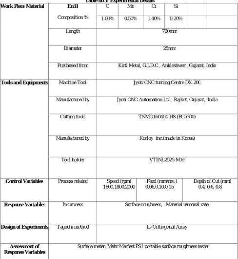
III. WORKPIECE, CUTTING TOOL USED AND EXPERIMENTAL DETAILS Table no.1: Experimental Details

Work Piece Material En31

Composition %

C Mn Cr Si

1.00% 0.50% 1.40% 0.20%

Length 700mm

Diameter 25mm

Purchased from Kirti Metal, G.I.D.C , Ankleshwer , Gujarat, India

Tools and Equipments Machine Tool Jyoti CNC turning Centre DX 200

Manufactured by Jyoti CNC Automation Ltd , Rajkot, Gujarat, India

Cutting tools TNMG160404-HS (PC5300)

Manufactured by Korloy inc.(made in Korea)

Tool holder VTJNL2525 M16

Control Variables Process related Speed (rpm) 1600,1800,2000

Feed (mm/rev.) 0.06,0.10,0.15

Depth of Cut (mm) 0.4, 0.6, 0.8

Response Variables In-process Surface roughness, Material removal rate.

Design of Experiments Taguchi method L9 Orthogonal Array

Assessment of Response Variables

(4)

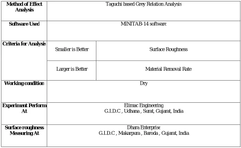
Copyright to IJIRSET DOI:10.15680/IJIRSET.2016.0507118 12700 Method of Effect

Analysis

Taguchi based Grey Relation Analysis

Software Used MINITAB-14 software

Criteria for Analysis

Smaller is Better Surface Roughness

Larger is Better Material Removal Rate

Working condition Dry

Experiment Perform At

Elimac Engineering

G.I.D.C , Udhana , Surat, Gujarat, India

Surface roughness Measuring At

Dhara Enterprise

G.I.D.C , Makarpura , Baroda , Gujarat, India

IV. EXPERIMENTATION

A. Selection of parameter

Table no.2 Selection of parameter

Input Variable Level 1 Level 2 Level 3

Speed(rpm) 1600 1800 2000

Feed(mm\rev) 0.06 0.10 0.15

Depth of cut(mm) 0.4 0.6 0.8

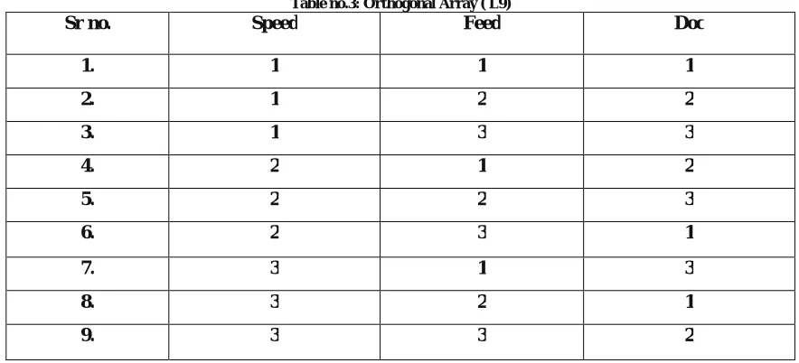
B. Selection of Orthogonal Array:

(5)

Table no.3: Orthogonal Array ( L9)

Sr no. Speed Feed Doc

1. 1 1 1

2. 1 2 2

3. 1 3 3

4. 2 1 2

5. 2 2 3

6. 2 3 1

7. 3 1 3

8. 3 2 1

9. 3 3 2

C. Experiment Result

The experiments were conducted, with the process parameter levels set as given in Table 7, to study the effect of

process parameters over the output parameters. Experiments were conducted according to the test conditions specified by the Taguchi design. Experimental results are given in Table for surface roughness (Ra), material removal rate (MRR) Altogether 9 experiments were conducted using Taguchi method.

Sr no.

Control parameter Response parameter

Speed (rpm)

Feed (mm\rev)

Depth of cut (mm)

MRR (mm3\min.)

(Ra)µm

1

1600

0.06 0.4 1389.79 2.0835

2 1600 0.10 0.6 3057.49 1.7502

3 1600 0.15 0.8 5504.06 1.3705

4 1800 0.06 0.6 2183.98 2.088

5 1800 0.10 0.8 4299.63 1.3805

6 1800 0.15 0.4 2866.24 1.6422

7 2000 0.06 0.8 3227.17 1.1372

8 2000 0.10 0.4 2457.12 1.796

(6)

V. DATA ANALYSIS & RESULTS DISCUSSION A. Taguchi Based Grey Relation Analysis

Grey analysis is a new technology, a group of techniques for system analysis and modeling. It is also called grey logic or grey system theory. Grey analysis is useful in situations with incomplete and uncertain information. Grey analysis is particularly applicable in instances with very limited data and in cases with little system knowledge or understanding. Grey analysis was invented by Professor Deng Julong of the Huazhong University of science and Technology in Wuhan, China. Grey analysis has been successfully used in a wide range of fields diverse as agriculture, ecology, economic planning and forecasting, traffic planning, industrial planning and analysis, management and decision making, irrigation strategy, crop yield forecasting, military affairs, target tracking, population control, communication system design, geology, oil exploration, earthquake prediction, material science, manufacturing, biological protection, environmental impact studies, medical management and the judicial system.

According to grey analysis proponents, different grey analysis elements are applicable to all systems. Grey relational analysis is an improved method for identifying and prioritizing key system factors, provides a straightforward mechanism for proposal evaluations and is useful for variable independence analysis

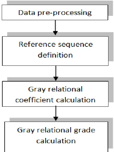
Steps for Grey Relational Analysis (GRA)

GRA is effective tool for solving the complicated interrelationship among the designated performance characteristics. It also provides an efficient solution to multi-input and discrete data problems. In grey relational analysis the complex multiple response optimization problem can be simplified into optimization of single response grey relational grade. The procedure for determining the grey relational grade is represented graphically in Fig. no.1 and discussed below

(7)

Step 1 Data pre-processing:

If the number of experiments is “m” and the number of response is “n” then the ith experiment can be expressed as Yi

= (yi1, yi2, ….., yij, ….., yin) in decision matrix form, where yij is the performance value (or measure of performance) of

response j (j = 1, 2, ….., n) for experiment i (i = 1, 2, ….., m). The general form of decision matrix D is given as,















mn mj ml in ij il n j l

y

D

...

1 1

1

The term Yi can be translated into the comparability sequence Xi = (xi1, xi2… xij… xin) where xij is the normalized value

of yij for the response j (j = 1, 2… n) of experiment i (i = 1, 2… m). After normalization, decision matrix D becomes

normalization matrix D’ is given as follows.















mn mj ml in ij il n j l

x

D

...

'

1 1 1

The normalized values xij are determined by use of following equation. There are for beneficial type, non-beneficial

type and target value type responses.

1. If the expectancy of the response is larger-the-better (i.e. beneficial response), then it can be expressed by

2. If the expectancy of the response is smaller-the-better (i.e. non-beneficial response), then it can be expressed by

3. If the expectancy of the response is nominal-the-best (i.e. closer to the desired value or target value), then it can be expressed by

where Yj* is closer to the desired value of jthresponse.

(3)

(1)

(8)

Copyright to IJIRSET DOI:10.15680/IJIRSET.2016.0507118 12704 Table no. 5: Signal to Noise Ratio

Sr. no

MRR (mm3\min.)

Surface roughness(Ra)µm

S\N Ratio(MRR) S\N Ratio(Ra)

1 1389.79 2.0835 62.8589 -6.3758

2 3057.49 1.7502 69.7059 -4.8617

3 5504.06 1.3705 74.8136 -2.7375

4 2183.98 2.088 66.784 -6.3946

5 4299.63 1.3805 72.66 -2.8007

6 2866.24 1.6422 69.146 -4.3085

7 3227.17 1.1372 70.176 -1.1167

8 2457.12 1.796 67.808 -5.0861

9 4517.32 1.02675 73.0976 -0.2292

Step 1: Normalised Data

Table no 6: Normalised Data

Sr. no Speed (rpm)

Feed (mm\rev)

Doc (mm)

Normalised data(MRR)

Normalised data(Ra)

1 1600 0.06 0.4 0 0.00424

2 1600 0.10 0.6 0.405345 0.318289

3 1600 0.15 0.8 1 0.676058

4 1800 0.06 0.6 0.193033 0

5 1800 0.10 0.8 0.707255 0.666635

6 1800 0.15 0.4 0.358861 0.420051

7 2000 0.06 0.8 0.446587 0.895882

8 2000 0.10 0.4 0.259421 0.275134

(9)

Step 2 Deviation sequence:

In comparability sequence all performance values are scaled to [0, 1]. For a response j of experiment i, if the value xij

which has been processed by data pre-processing procedure is equal to 1 or nearer to 1 then the value for any experiment, then the performance of experiment i is considered as best for the response j. The reference sequence Xis defined as (x1, x2, ….., xj, ….., xn) = (1, 1, ….., 1, …..,, 1), where xjis the reference value for jth response and it aims to

find the experiment whose comparability sequence is closest to the reference sequence.

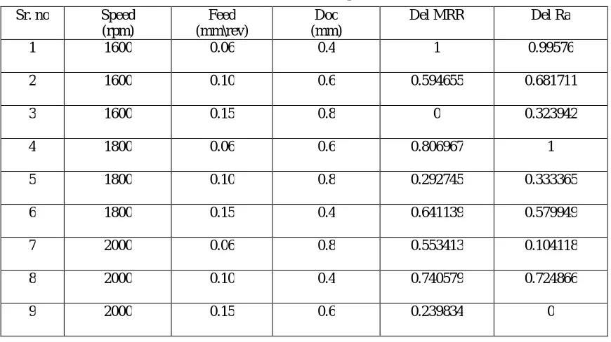
Step 2: Deviation Sequences

Table no 7: Deviation Sequences

Sr. no Speed (rpm)

Feed (mm\rev)

Doc (mm)

Del MRR Del Ra

1 1600 0.06 0.4 1 0.99576

2 1600 0.10 0.6 0.594655 0.681711

3 1600 0.15 0.8 0 0.323942

4 1800 0.06 0.6 0.806967 1

5 1800 0.10 0.8 0.292745 0.333365

6 1800 0.15 0.4 0.641139 0.579949

7 2000 0.06 0.8 0.553413 0.104118

8 2000 0.10 0.4 0.740579 0.724866

9 2000 0.15 0.6 0.239834 0

Step 3 Grey relational coefficients:

Grey relational coefficient is used for determining how close xij is to xj. The larger the grey relational coefficient, the

closer xij and xj are. The grey relational coefficient can be calculated by using following equation.

For i = 1, 2… m and j = 1, 2... n Where, = the grey relational coefficient between xij and x0j

(10)

D min = min {D ij, I 1, 2... m; j= 1, 2… n} D max = max {D ij, I 1, 2... m; j= 1, 2… n}

Distinguishing coefficient (ζ) is also known as the index for distinguish ability. The smaller distinguishing coefficient is, the higher is its distinguishing ability. It represents the equation’s “Contrast Control”. The purpose of distinguishing coefficient is to expand or compressed the range of the grey relational coefficient. Different distinguishing coefficient may lead to different solution results. Decision makers should try several different distinguishing coefficients and analyze the impact on GRA results. Considering value of distinguishing coefficient is 1

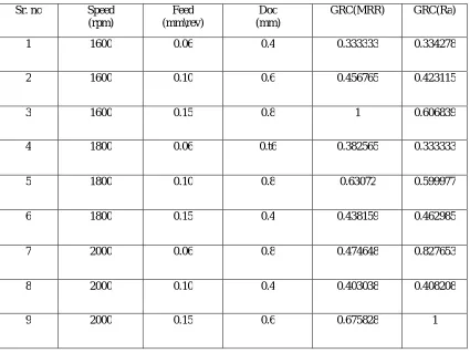
Step 3: : Grey Relation co-efficient

Table no. 8: Grey Relation co-efficient

Sr. no Speed

(rpm)

Feed (mm\rev)

Doc (mm)

GRC(MRR) GRC(Ra)

1 1600 0.06 0.4 0.333333 0.334278

2 1600 0.10 0.6 0.456765 0.423115

3 1600 0.15 0.8 1 0.606839

4 1800 0.06 0.t6 0.382565 0.333333

5 1800 0.10 0.8 0.63072 0.599977

6 1800 0.15 0.4 0.438159 0.462985

7 2000 0.06 0.8 0.474648 0.827653

8 2000 0.10 0.4 0.403038 0.408208

(11)

Step 4 Grey relational grades:

The measurement formula for quantification in grey relational space is called grey relational grade. A grey relational grade (grey relational degree) is a weighted sum of grey relational coefficients and it can be calculated using following equation.

i

w

ij

n

j j



.

1





i = 1, 2… m and j = 1, 2… n ……… (5)

In above equation



i is the grey relational grade between comparability sequence Xi and reference sequence Xn. It represents correlation between the reference sequence and the comparability sequence. wj is the weight of response

surface j and depends on decision maker’s judgment.

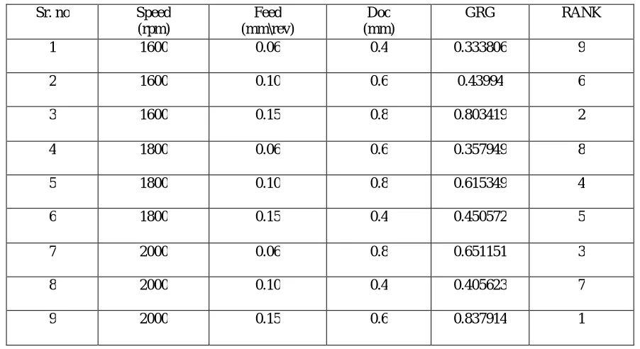
Step 4: Grey Relation Grade

Table no.9: Grey Relation Grade

Sr. no Speed

(rpm)

Feed (mm\rev)

Doc (mm)

GRG RANK

1 1600 0.06 0.4 0.333806 9

2 1600 0.10 0.6 0.43994 6

3 1600 0.15 0.8 0.803419 2

4 1800 0.06 0.6 0.357949 8

5 1800 0.10 0.8 0.615349 4

6 1800 0.15 0.4 0.450572 5

7 2000 0.06 0.8 0.651151 3

8 2000 0.10 0.4 0.405623 7

9 2000 0.15 0.6 0.837914 1

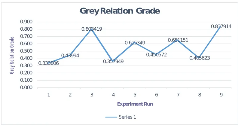
B. Result

(12)

Copyright to IJIRSET DOI:10.15680/IJIRSET.2016.0507118 12708 Fig no.2: Graph of Grey Relation Grade

Figure no 3 : Main Effect Plot for Ra

2000 1800 1600 1.8 1.6 1.4 0.15 0.10 0.06 0.8 0.6 0.4 1.8 1.6 1.4 Speed (RPM) M e a n o f M e a n s Feed (mm/rev.)

Dept h of Cut (mm)

Main Effects Plot for Means of Roughness

Data Means 0.333806 0.43994 0.803419 0.357949 0.615349 0.450572 0.651151 0.405623 0.837914 0.000 0.100 0.200 0.300 0.400 0.500 0.600 0.700 0.800 0.900

1 2 3 4 5 6 7 8 9

G re y R el at io n G ra de Experiment Run

Grey Relation Grade

(13)

Figure no 4 : Main Effect Plot for MRR

2000 1800

1600 4000

3500

3000

2500

2000

0.15 0.10

0.06

0.8 0.6

0.4 4000

3500

3000

2500

2000

Speed (RPM)

M

e

a

n

o

f

M

e

a

n

s

Feed (mm/rev.)

Depth of Cut (mm)

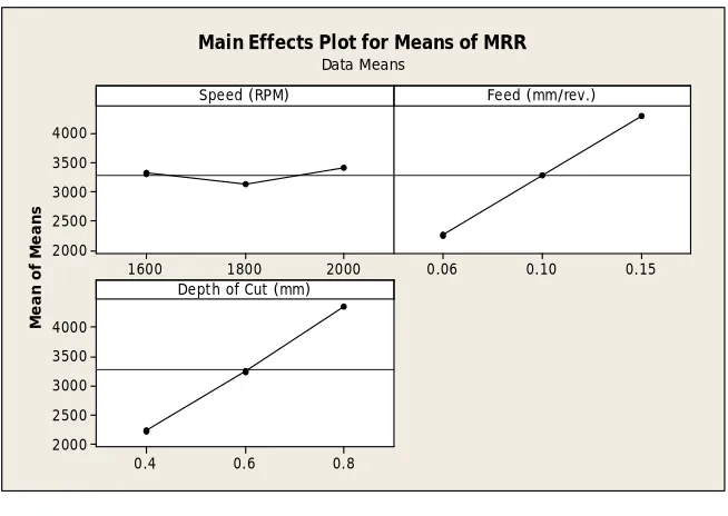
Main Effects Plot for Means of MRR

Data Means

V. CONCLUSION

This paper presents research work of the optimal combination of various cutting parameters affecting the surface roughness, material removal rate in Dry turning of EN31 material by using PVD coated carbide tools. An orthogonal array with grey relational analysis was used to optimize the multi response characteristics of the EN31 turning process. The performance characteristics such as the minimum surface roughness and maximum material removal rate were improved using the method proposed in this study. According to the Taguchi L9 Orthogonal array, 9 experiment need to be conducted to find the optimal parameter conditions at three levels, three control factor en31 turning. Grey relational analysis found that the feed is the most influencing factors for surface roughness and speed and depth of cut are most influencing factors for Material removal rate. The optimal parameter combinations obtained by the analysis is at Speed 2000 rpm, Feed 0.15 mm/rev, Depth of cut 0.6 mm. The experiment value is also very closer to predicted value .The highest grey relation grade is 0.837914.

REFERENCES

[1] Ashok Kumar Sahoo, Achyuta Nanda Baral, Arun Kumar Rout, B.C. Routra, “Multi-objective optimization and predictive modelling of surface roughness and material removal rate in turning using Grey Relational and Regression Analysis”, Procedia Engineering, Vol. 38, pp. 1606-1627,2012

[2] Chorng-Jyh Tzeng, Yu-Hsin Lin, Yung-Kuang Yang, Ming-Chang Jeng, “Optimization of turning operations with multiple performance characteristics using the Taguchi method and Grey relational analysis”, Journal of Materials Processing Technology, 209 ,pp. 2753-2759.,2012

[3] J Nithyanandam, Sushil Laldas, K Palanikumar, “Surface roughness analysis in turning of titanium alloy by nano coated carbide insert” Procedia Materials Science,Vol,.3Issue no 6, pp.2159 – 2168, 2014.

[4] Sudhansu Ranjan Das, Amaresh Kumar, and Debabrata Dhupal, “Effect of Machining Parameters on Surface Roughness in Machining of Hardened AISI 4340 Steel Using Coated Carbide Inserts”, International Journal of Innovation and Applied Studies, Vol. 2, pp. 445-453, 2013. [5] Ajay Mishraa and Anshul Gangele , “ Multi-Objective Optimization In Turning Of Cylindrical Bars Of AISI 1045 Steel Through Taguchi’s Method And Utility concept”, International Journal of Sciences, Basic and Applied Research, Vol. 12, pp 28-36, 2013

[6] Reddy Sreenivasulu and Srinivasa Rao, “Design of Experiments based Grey Relational Analysis in Various Machining Processes - A Review” , Research Journal of Engineering science, Vol. 2(1), pp. 21-26,2013.

[7] A. Ersan Aslan, Necip Causcu,Burak Birgoren, “Design Optimization Of Cutting Parameters When Turning Hardened AISI 4140 Steel (63 HRC) With Al2O3+ TiCN Mixed Ceramic Tool”,Material and Design ,Vol. 28, pp.1618-1622, 2006

[8] J. Laxman, Dr. K. Guru Raj, “Optimization of EDM Process Parameters on Titanium Super Alloys Based on the Grey Relational Analysis” International Journal of Engineering Research, Volume No.3, Issue No.5, pp. 344-348, 2013.