The Coalescent in a Continuous, Finite, Linear Population
Jon F. Wilkins*
,1and John Wakeley
†*Program in Biophysics and†Department of Organismic and Evolutionary Biology, Harvard University, Cambridge, Massachusetts 02138
Manuscript received June 10, 2001 Accepted for publication March 4, 2002
ABSTRACT
In this article we present a model for analyzing patterns of genetic diversity in a continuous, finite, linear habitat with restricted gene flow. The distribution of coalescent times and locations is derived for a pair of sequences sampled from arbitrary locations along the habitat. The results for mean time to coalescence are compared to simulated data. As expected, mean time to common ancestry increases with the distance separating the two sequences. Additionally, this mean time is greater near the center of the habitat than near the ends. In the distant past, lineages that have not undergone coalescence are more likely to have been at opposite ends of the population range, whereas coalescent events in the distant past are biased toward the center. All of these effects are more pronounced when gene flow is more limited. The pattern of pairwise nucleotide differences predicted by the model is compared to data collected from sardine populations. The sardine data are used to illustrate how demographic parameters can be estimated using the model.
M
IGRATION often plays an important role in shap- common ancestor of two or more sequences, rather than on the properties of the population as a whole. ing patterns of genetic diversity. Undercondi-tions of restricted gene flow, the geographical and genetic This focus on the genealogical structure of a sample provides a framework in which properties of popula-structures of a population tend to become correlated.
In the most basic terms, we expect individuals in close tions can be estimated. Coalescent theory applied to geographically structured populations with discrete geographical proximity to be genetically more similar
than geographically distant individuals. This differentia- demes has been formalized as the “structured coales-cent” (see,e.g.,Wilkinson-Herbots1998).
tion will arise even in the absence of local adaptation,
due to locally occurring genetic drift. As a result, it The coalescent model developed in this article as-sumes a population distributed uniformly along a finite, is possible to use existing patterns of neutral genetic
variation to make inferences about the geographic struc- one-dimensional habitat. Gene flow is restricted, so loca-tions of parents and offspring are correlated. A diffusion ture of populations.
The best-studied models of geographic structure are approximation is used to characterize the locations of ancestors of sampled sequences. Applied to pairs of the island (Wright1931;Maruyama1970a) and
step-ping-stone (Kimura and Weiss 1964) models. Both sequences, this approach fully specifies the probability density for the times and locations of their most recent types of model assume a population composed of a
common ancestors and also provides summary statistics number of subpopulations, or demes, connected to
such as the mean time to coalescence. each other through migration. Each deme is assumed
The model is analogous to the one-dimensional step-to be panmictic. In the island model, there is no explicit
ping-stone model, but with some important differences geography, in that each migration event occurs via a
that illustrate the motivation for this work. Although common migrant pool. Stepping-stone models, in
con-there has been a lot of work on finite stepping-stone trast, permit migration only between neighboring
models (discussed below), most analyses of the stepping-demes. In the one-dimensional model, the demes are
stone model rely on nonrealistic treatments of habitat arrayed in a line, and each deme exchanges migrants
boundaries. The best-studied models fall into two cate-only with the two adjacent demes. The analogous
two-gories. Models in the first category assume that the ends dimensional model assumes a grid of demes, with each
of the array are joined together (the circular stepping-deme exchanging migrants with some number of
neigh-stone model, or the toroidal model in two dimensions; bors (e.g., four).
e.g., Maruyama 1970b; Nagylaki 1974a, 1977;
Stro-Coalescent theory differs from classical population
beck 1987; Slatkin 1991). This assumption secures genetics in its focus on the time to the most recent
mathematical tractability by making all demes identical and migration isotropic (Strobeck1987), but is directly applicable to few systems in nature (e.g., a population
1Corresponding author:Harvard University, Biological
Laboratories-inhabiting the entire coast of an island). Models in the
2102, 16 Divinity Ave., Cambridge, MA 02138.
E-mail: [email protected] second category assume a linear habitat of infinite
length (e.g.,WeissandKimura1965;Nagylaki1974b, distribution of coalescence times (Slatkin1991), many classical population-genetic analyses do not make use 1976;Sawyer1976, 1977). While these models provide
of all of the information in DNA sequence data, making useful insights regarding the short-term behavior of
the coalescent approach presented here preferable. Fur-populations in a one-dimensional habitat, they predict
thermore, all of these analyses rely on approximations infinite divergence between individuals (Sawyer1976;
that assume a large local population size, an assumption
Griffiths1981;Wilkinson-Herbots 1998).
that is relaxed in the present analysis. However, it is The model studied here assumes a finite linear habitat
noteworthy that the results derived here are consistent (e.g., along a stretch of coastline). The analysis indicates
with, and in some cases anticipated by, much of this that the expected pattern of genetic diversity does, in
previous work. fact, depend on location in the habitat, suggesting that
A model similar to the one presented here was pro-application of a circular model to a finite linear
popula-posed by Barton andWilson (1995, 1996), who ap-tion is problematic. At the very least, this misapplicaap-tion
plied a coalescent approach to a continuous population entails discarding information encoded in the variation
in two dimensions, deriving recursion equations that in genetic diversity along the population range.
describe the coalescent process for a pair of sequences. Models of isolation by distance in a continuous
popu-These equations agree closely with simulated distribu-lation date back to Wright (1943), who defined the
tions of coalescence times. However, the method be-effective neighborhood population size as the reciprocal
comes cumbersome for long coalescence times and does of the probability of self-fertilization. That is, the
neigh-not readily lead to summary statistics such as the mo-borhood size is approximately the number of individuals
ments of the probability distribution. While limited to within the single-generation dispersal range. Wright’s
pairs of genes in a one-dimensional habitat, the model work shows that the correlation between adjacent
indi-presented here is easily applied to both long and short viduals and the differentiation between neighborhoods
coalescence times and yields summary statistics that can both increase as the neighborhood size becomes small
be used to make inferences regarding demographic his-compared with the total population size. However,
tory from genetic data. Simulation results confirm that much of the theoretical work since has focused on
popu-the diffusion approximation used in this model provides lations subdivided into discrete demes. While a discrete
an accurate characterization of the entire coalescent model may be appropriate for many organisms, others
process under a broad range of parameter values. may be distributed more or less continuously across
a particular range, but nevertheless be geographically
structured due to limited gene flow. The model pre- THE MODEL
sented here assumes a continuous population, but can
The model assumes a uniformly distributed popula-be applied in modified form to the discrete-demes
tion ofNhaploid individuals in a linear habitat, but can model.
be applied to a population ofN/2 diploid individuals Work from within the classical population genetics
without modification. Distance is scaled such that any paradigm provides some insight to the properties of
location along the habitat is indexed by a number be-finite linear models similar to the one considered here.
tween 0 and 1 (with1⁄
2being the midpoint of the
habi-Finite one-dimensional stepping-stone models have tat). Absolute density-dependent population regulation been analyzed byMaruyama(1970c),FlemingandSu is assumed. Each individual occupies a space of width
(1974), and Male´cot (1975). These analyses derive 1/N, from which all other individuals are excluded. The expectations for classical measures such as the covari- structure of the population is a one-dimensional lattice, ance in gene frequencies across demes.Nagylakiand as in the voter model (HolleyandLiggett1975), a
Barcilon(1988) have considered probabilities of iden- contact-process model used in many ecological applica-tity in a semiinfinite linear habitat.Maruyama(1971) tions (DurrettandLevin 1994). The distribution of has also derived probabilities of identity for a continu- coalescence times is found using a continuous approxi-ous population on a torus and the rate of decrease in mation. Another way to think of the model is as a step-genetic variability in a finite two-dimensional popula- ping-stone model consisting ofNdemes, each of size 1. tion (Maruyama1970d, 1972). Hey(1991) has com- Generations are nonoverlapping. Each individual pared the mean coalescence time for a pair of sequences produces a very large number of gametes, which are sampled from opposite ends of a finite linear stepping dispersed according to a normal distribution centered stone with that of a pair sampled at random from the at the location of the individual and with variance entire population. The result that coalescence times are 22
m. Thus in each generation an effectively infinite
num-longer near the center of the habitat range is consistent ber of gametes arrives at each location. One of these with findings ofHerbots(1994, pp. 66 and 145–146), gametes is selected at random to become the adult at who found a similar pattern in linear stepping-stone that location in the next generation. The distribution
models with three and five demes. of the origins of those gametes is the correlation of the
Thus, the location of a parent is normally distributed around the location of its offspring, with variance 22
m
(a grandparent is normally distributed around the same location with variance 42
m, and so on).
The boundaries of the habitat are reflecting, so a gamete that would otherwise land outside the habitat range is reflected back an equal distance within it. Each individual thus has the same expected number of off-spring regardless of its location. This means that migra-tion is conservative, so migramigra-tion alone is sufficient to maintain the relative population densities at all loca-tions in the habitat (Nagylaki 1980). Nonreflecting boundaries would correspond to the case where those gametes dispersing outside the habitat range are lost. In such a system, individuals near the edges of the habitat would have a reduced effective fecundity relative to those nearer to the center.
AsFelsenstein(1975) pointed out, most continuous-space models in population genetics assume a uniform population density that would not actually be main-tained by the proposed reproductive scheme. A normal
Figure 1.—The diffusion process for two lineages. The
distribution of gametes without severe density regula- graphs illustrate the process of lineage diffusion backward in tion generates a population that is clumped together time. (A) The probability distribution for the locations of the two lineages at a time in the recent past. For sequences
sam-at certain locsam-ations and sparsely populsam-ated sam-at others.
pled from different locations, there is little overlap in the two
With its absolute density regulation at all locations, the
distributions and therefore little possibility of a coalescent
model of reproduction proposed here will immediately event. Going farther back in the past (B and C), the overlap generate and maintain a population that is uniformly between the two distributions initially increases, and the prob-distributed across its habitat range. ability of the two sequences sharing a common ancestor in-creases. More recent coalescent events are most likely to occur
Applying a coalescent approach to the analysis of this
near the center of the space separating the two samples (B).
model involves tracking the location of the ancestors of
In the more distant past, the overlap between the two decreases
a particular sequence back in time. The location of a and broadens, and the range over which coalescent events single sampled lineage can be approximated using a are likely to have occurred becomes less well defined (C). diffusion process with diffusion constant2
m. The precise
location of a lineage is known only for the generation in which sampling occurred, so its location in the past
is represented here as a probability distribution. Consid- boundaries for the moment, it is equally likely to have ering only a single sequence sampled from a particular come from a location to its left or its right in the previous locationz0and its ancestors, one can imagine how this generation. It follows that when we consider two
lin-probability distribution broadens going back in time. eages at some distance from each other, they are equally In the distant past, the distribution becomes completely likely to have been closer together or farther apart in flat, when the ancestral sequence is equally likely to the previous generation. However, if the two shared a have been anywhere in the range. The exact distribution common ancestor in the previous generation, they must of ancestral locations can be derived for such a system have been closer together. Thus, conditional on not
using a Fourier series. coalescing in the previous generation, the two lineages
The analysis presented here derives the distribution are slightly more likely to have been farther apart than of the time to coalescence for a pair of sequences drawn closer together. In contrast to the single-sequence case, from locationsz0
1andz02in the habitat. Each lineage is as time in the past becomes very large, the ancestral
subject to a diffusion process backward in time, with lineages are not equally likely to be found anywhere in the probability of coalescence related to the overlap of the habitat range. If the two lineages are still distinct, the two probability distributions (Figure 1). The solu- they are likely to have been more geographically sepa-tion employs a two-dimensional Fourier method, but is rated than a uniform distribution dictates.
The analysis involves a transformation of variables to more complicated than the case of a single sequence
because the ancestral location distributions z1(t) and create two new parameters that do diffuse
indepen-dently. The first parameter encodes the distance be-z2(t), conditional on not yet having coalesced, are not
independent of each other. tween the two sequences, and the second their average
more complex, partially reflecting, partially absorbing boundary. Positions along this line represent states where the two ancestral lineages are very close together in space. Reflection is equivalent to the two lineages moving past each other. Absorption is equivalent to a coalescent event.
The diffusion process in the transformed state space is isotropic, but not separable. Although diffusion in one dimension is independent of diffusion in the other dimension, it is not independent of location, due to the fact that the state space is triangular. The diagonal reflecting boundaries can be eliminated by placing a mirror image of the state space opposite the boundary. Reflection at the boundary is now represented as move-ment into the mirror-image state space. Three such reflections transform the state space into a square rang-ing from ⫺1 to 1 in bothx and y. All four edges are Figure2.—The state space of the system in the transformed
coalescent boundaries, and the symmetric shape makes
coordinates. Diffusion of the two lineages in the
one-dimen-thexandydiffusion processes separable as
sional habitat is represented as the diffusion of a single point in a two-dimensional state space. Thexcoordinate encodes the
U(x,y,t)⫽Ux(x,t)Uy(y,t), (4) distance between the two lineages, withx⫽0 corresponding to
the maximal separation of the two andx⫽1 corresponding to
where each distribution satisfies the diffusion equation
the two lineages being at the same location. Theycoordinate encodes the average position of the two lineages, withy⫽ ⫺1
corresponding to both lineages being at the end of the range Ux
t ⫽ 2
2 m
2U
x
x2 (5)
where z⫽ 0 and y⫽ 1 corresponding to z⫽1. The point
x⫽0,y⫽0 is at the center of the square that is generated
by the three reflections. Uy
t ⫽ 2
2 m
2U
y
y2. (6)
Each pair of locations (z1,z2) in the real habitat
corre-sponds to four locations in this square space, one in
x⫽1⫺|z1⫺z2| (1) each of the four images of the triangular state space
(see Equation A40). y⫽z1 ⫹z2⫺1. (2)
The boundary conditions at the edges of the square The “1” terms in Equations 1 and 2 are included for depend on both the population density and the dis-mathematical convenience, and other coordinate sys- persal (migration) rate. If the population density and tems would yield the same results, so long as diffusion dispersal rate are very high, then when the two lineages is isotropic. The distribution of ancestral locations t come close together, they are likely to pass by each other generations in the past can now be represented as a rather than share a common ancestor, because there two-dimensional probability surface inxandy: are a large number of individuals within their dispersal range. This corresponds to a more reflecting boundary
U(x,y,t). (3) in the two-dimensional state space. On the other hand,
if the population density and dispersal rate are low, This probability distribution is nonzero within a right neighborhood size is small, and two lineages that are triangle ranging from⫺1 to 1 inyand from |y| to 1 in close together in space will be more likely to share a
x(Figure 2). common ancestor, corresponding to a more absorbing
The genealogical history is now modeled as a single boundary. Mathematically speaking, the flux rate of the diffusion process in this triangular state space. The diffu- probability distribution across the boundary is equal to sion constant is 22
m, twice that for the single-particle the probability that the two lineages coalesce in the
diffusion process discussed above. This factor of two previous generation.
arises from the fact that the new parameters are the Because the model assumes perfect density-depen-sum and difference of two2
m single-particle diffusion dent population regulation, there is exactly one haploid
processes. lineage in each span of width 1/N.A coalescent event
physical separation of zero, which leads to pathological a simple form analogous to that for the expectation (Equations A26–A31 and A34). It is also possible to behaviors when applied to models of more than one
dimension. In our continuous approximation of the write down the exact distribution of the locations of two lineages that have not yet coalesced (A40), as well as population, we assume that a coalescent event occurs
whenever the two lineages are separated by a distance the distribution of locations of the coalescent events (A44–A46).
of⬍1/(2N), that is, when 1⫺1/(2N)⬍ x⬍ 1. This approximates the probability that both lineages are found within the same fixed span of width 1/N.
RESULTS
Applying this criterion at the boundaries, the result is
an infinite series of sine and cosine terms. The full The results derived in this article have been compared to simulation data to assess the accuracy of the diffusion solution is derived in theappendix, and the main results
are reproduced here in the text. For example, the joint approximation in this context. This section contains analytic and simulation results for a number of values probability density for the locations of the two lineages
is given by over a range of parameters. These results provide both
reassurance regarding the accuracy of the equations and insight into the behavior of the coalescent process Ux(x,t)⫽
兺
∞
i⫽1
␣ifi(x0)cos(␣ix)
␣i ⫹sin(␣i)cos(␣i)e ⫺22
m␣2i(t⫺1/2)
in a continuous, linear habitat.
Monte Carlo simulations were performed backward
⫹
兺
∞j⫽1
␣*j f*j (x0)sin(␣*j x) ␣*j ⫺sin(␣*j )cos(␣*j )
e⫺22m␣*2j(t⫺1/2) (7)
in time using two different migration/coalescence pro-cesses. In the first process, the locations of the two lin-eages were kept as floating point numbers. Migration Uy(y,t)⫽
兺
∞
i⫽1
␣ifi(y0)cos(␣iy)
␣i⫹sin(␣i)cos(␣i)e ⫺22
m␣2i(t⫺1/2) each generation was performed by drawing a random number from a normal distribution. If the new location for the lineage lay outside the habitat range, the new
⫹
兺
∞j⫽1
␣*j f*j (y0)sin(␣*j y) ␣*j ⫺ sin(␣*j)cos(␣*j )
e⫺22m␣*2j(t⫺1/2). (8)
location was selected by reflection at the habitat bound-ary. A coalescent event occurs if, after translocation and reflection, the two lineages lie within a distance 1/(2N) These series can be truncated for purposes of making
of each other. Times and locations of coalescent events calculations without significant loss of accuracy. The␣i
were averaged over a large number of sample runs. and␣*j terms are determined by the boundary
condi-The second process used a discrete lattice model. tions (see Equations A13), and thefiandf*j terms are
Each of the two lineages was assigned an integer location determined by the two sampling locations (Equations
between 1 andN.Each generation two pseudorandom A21). Discussion of Fourier-series solutions of the
diffu-integers were drawn from independent Poisson distribu-sion equation can be found in most texts (e.g.,
tions for each lineage, which were then translocated by
ChurchillandBrown1987). The treatment of initial
the difference of the two Poissons. This produces a conditions used here is standard, and the boundary
discrete distribution that approximates the shape of a conditions are incorporated using the Sturm-Liouville
normal distribution. Reflections were performed as in method.
the first process. If, after migration and reflection, the At timet, the probability of the two lineages not yet
two lineages were at the same location (had the same having coalesced is equal to the volume under the
prob-integer location value), a coalescent event was consid-ability surface defined byU (x,y,t) within the square
ered to have occurred. Again, the times and locations
⫺1⬍ x⬍ 1,⫺1⬍ y ⬍ 1. Intuitively, this is because
of the coalescent events were averaged over a large num-coalescence is represented by the diffusion of the
proba-ber of sample runs. bility density out of the square. Thus, the instantaneous
The relative value of the mean time to coalescence rate of coalescence at timetis given by the rate at which
is determined largely by the productN2
m, which is
analo-the probability volume within analo-the square is decreasing
gous to Nm in discrete-deme models of geographical at that time. From this relationship it is possible to derive
structure. Presented here are three sets of data repre-the expectation of repre-the time to coalescence for two
se-senting three different values ofN2
m. In all three cases
quences sampled from locations corresponding to x0
N⫽200. The values of2
mare 0.005, 0.0005, and 0.00005
andy0:
(N2
m⫽ 1.0, 0.1, and 0.01). For each value of2m, the E[T]⫽1
2⫹
兺
i兺
j2 2
m(␣2i⫹ ␣2j)
sin(␣i)fi(x0)
␣i⫹sin(␣i)cos(␣i)
sin(␣j)fj(y0)
␣j⫹sin(␣j)cos(␣j)
. mean time to coalescence was determined for a pair of sequences for a number of sampling locations. Figure (9)
3 presents mean time to coalescence determined analyti-cally from Equation 9 for the parameters used in Table It is possible using this approach to derive a number
of other analytic results, including the full probability 2 (N2
m⫽ 0.1). Mean times to coalescence in Tables 1–3
are determined by three methods. The first two values distribution for the time to coalescence (Equations A25
meth-reflecting boundary (Maruyama1970c;Nagylakiand
Barcilon1988) and by the work ofHerbots(1994). The model also provides results regarding the loca-tions of the lineages and common ancestors (Equaloca-tions A40–A46). Figure 4 shows the probability surface for the time and location of coalescence for three different pairs of sequences (from Equation A44). Recent coales-cent events are likely to be found in the region between the two sampling sites. In the more distant past, the probability distribution depends only on the migration rate and not the sampling locations. This distant-past distribution is biased toward the center of the range. Another result that can be derived from the model is the distribution of the lineage locations conditional on their still being separate at a timetin the past (Equation A40). In the distant past, this distribution is skewed toward the edges. Intuitively, if the two lineages are separated by a very deep genealogical branch, it most likely results from their having spent a lot of time at oppo-Figure3.—This surface represents the mean coalescence
times for pairs of sequences drawn from various locations site ends of the range. A number of other results are also
in the habitat range. The data here are equivalent to those derived and presented in the appendix, including the
presented in Table 2 (N⫽100,2
m⫽0.001). Thex- andy-axes strong-migration limit (Nagylaki1980, 2000) and
appli-represent the two sampling locations. Darker areas correspond
cation of these results to a linear array of demes.
to shorter mean coalescence times. The lower-left and upper-right corners represent the case where both samples are taken from one end of the range. The other two corners (with the
APPLICATION TO DATA longest coalescence times) represent the case where the two
samples are taken from opposite ends of the range. Mean The expected time to coalescence can be used to
coalescence times are longer for samples taken from the
cen-estimate demographic parameters. In this section
pub-ter of the array than for samples taken from near the ends.
lished sequence data are used to fit the model and estimate the effective population size and the genetic dispersal rate. Our purpose here is not to determine ods described above) from 1 million replicates. The
specific parameter values for a particular organism. In third value is the analytically determined value from
fact, the population considered below is likely to violate Equation 9.
one or more assumptions of the model. Our goal is Inspection of the tables reveals that the analytically
simply to illustrate the fact that patterns of genetic diver-derived mean time to coalescence is in good agreement
sity such as the one predicted by the model may be with simulated data, with the results of the three
meth-found in nature. We also want to emphasize the fact ods differing typically by no more than 0.5%. Tables
that the finite linear model makes different predictions 1–3 and Figure 3 also immediately reveal two features
under neutrality than either an island or a circular of this model. First is the intuitively pleasing result that model and that these differences may alter our interpre-the mean time to coalescence increases with interpre-the physical tation of sequence data.
distance between the two sampled sequences. The rate We have applied the model developed here to se-of increase with distance is dependent on the migration quence data collected from the mitochondrial control rate, with lower migration rates corresponding to higher region in the five different regional forms of sardines
rates of genetic divergence with distance. (Sardinops) in the Indian and Pacific oceans (Bowen
A second, less intuitive, result from these data is the and Grant 1997). Sardines are characterized by an dependence of time to coalescence on the location of antitropical distribution and are restricted to five tem-the two sampled sequences (in contrast to tem-their separa- perate upwelling zones off the coasts of Japan, Califor-tion). The pattern is most easily seen by considering nia, Chile, Australia, and South Africa. Temperate wa-pairs of adjacent sequences sampled from various loca- ters extend continuously from South Africa through tions along the habitat. A pair of adjacent sequences Australia to Chile and from Japan to North America. sampled from the center of the population range has The two temperate zones are separated by warmer tropi-a longer metropi-an time to cotropi-alescence thtropi-an ptropi-airs stropi-ampled cal waters in the Pacific. However,BowenandGrant
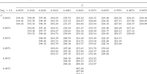
TABLE 1
Comparison of derived and simulated mean coalescence times (N⫽100;2
m⫽0.0001)
z0 2
N2
m⫽0.01 0.0075 0.1025 0.2025 0.3025 0.4025 0.5025 0.5975 0.6975 0.7975 0.8975 0.9975
z0 1
0.0025 36.60 281.68 669.21 1113.47 1570.23 2001.93 2371.48 2668.08 2932.13 3078.44 3133.22
37.47 279.72 667.07 1110.76 1569.15 1995.55 2364.42 2684.84 2926.59 3079.56 3129.56
37.41 280.99 669.28 1113.92 1568.95 2001.45 2368.60 2690.41 2931.44 3081.25 3133.56
0.0975 141.70 549.87 1014.72 1487.27 1928.50 2305.56 2632.17 2878.58 3032.74
141.72 548.70 1014.94 1484.19 1929.06 2306.08 2630.55 2883.32 3033.48
142.65 549.32 1014.88 1485.21 1929.46 2305.30 2634.11 2880.09 3032.88
0.1975 206.42 712.98 1226.90 1705.66 2112.37 2460.49 2727.98
204.91 709.88 1224.66 1706.43 2110.57 2460.18 2720.40
206.29 712.63 1228.65 1708.52 2111.00 2461.33 2722.62
0.2975 245.53 809.11 1344.81 1794.98 2178.62
244.31 809.61 1343.76 1788.08 2173.63
244.74 808.97 1346.20 1792.28 2178.23
0.3975 264.38 852.93 1361.66
263.59 851.07 1363.00
265.72 854.03 1359.55
0.4975 273.02
271.91 272.41
Tables 1–3 present a comparison of analytically derived mean coalescence times with values determined by simulation. Row and column headings indicate the sampling locations for the two sequences, in terms of distance along the population range. The leftmost nonempty cell in each row represents the case of two adjacent sequences at various points along the habitat. Mean coalescence times are longer for pairs of sequences that are more distant, as expected, but also for pairs of sequences drawn from closer to the center of the range.
the western Pacific, the tropical zone is much broader, with distance and greater genetic diversity near the cen-ter of the habitat. The productN2
m was estimated to
making genetic exchange between Japan and Australia
unlikely. be 0.017, and(⫽2N) was estimated to be 1.64.
Assum-ing a per generation mutation rate ofⵑ7.5⫻ 10⫺6for
On the basis of these observations, it may be
reason-able to apply the finite, linear model to this system, the mitochondrial control region (on the basis of a divergence rate of 15% per million years between lin-treating the populations as linearly arrayed from Japan
to California to Chile to Australia to South Africa, with eages and a mean generation time of 2 years, Butler
et al. 1996), this gives a total mitochondrial effective genetic contact possible only between adjacent
popula-tions. The total length of this range isⵑ25,000 miles, population size of 2 ⫻ 105. This value is likely much
smaller than the census size, possibly resulting from a with the five sampling sites occurring at ⵑ5000-mile
intervals. These five sites yield 15 pairwise comparisons, higher variance of reproductive success than that as-sumed by the model and also consistent with suggestions which were fit to the model by finding the parameter
values that minimize the sum of the squares of the differ- of population fluctuations in the species (Soutarand
Isaacs1974). This produces an estimate of2
m⫽8.5⫻
ences between the predicted and observed values. The
statistical properties of these estimators are not investi- 10⫺8, which corresponds to a mean intergenerational
migration distance ofⵑ8 miles and a (mitochondrial) gated here. However, in this case, the model does
ap-pear to fit the data reasonably well, reproducing the neighborhood size ofⵑ200.
Inferences can also be drawn from differences in ob-same pattern of genetic diversity, and it provides a
framework that highlights certain features of the data. served and expected values. In the fourth column of Figure 5 (labeled “Calif.”), the observed interpopulation Figure 5 shows the observed and expected average
number of pairwise nucleotide differences (propor- values are all lower than the corresponding expected values. In the fifth column (“Japan”), on the other hand, tional to the expected coalescence time) in the data set
for parameter values minimizing the sum of the squares the expected values are lower than the observed. This pattern suggests that the California and Chile popula-of the errors. The observed data manifest the two key
TABLE 2
Comparison of derived and simulated mean coalescence times (N⫽100;2
m⫽0.001)
z0 2
N2
m⫽0.1 0.0075 0.1025 0.2025 0.3025 0.4025 0.5025 0.5975 0.6975 0.7975 0.8975 0.9975
z0 1
0.0025 119.82 163.96 223.05 280.07 333.74 381.82 421.42 454.09 478.93 494.39 499.97
120.64 163.78 223.23 280.18 333.85 382.85 420.77 454.56 479.53 494.62 499.57
120.25 164.58 223.64 281.02 334.57 382.57 421.76 455.20 479.78 494.87 500.11
0.0975 162.54 213.61 272.87 326.64 375.96 415.52 449.19 473.93 489.99
162.57 214.46 272.85 327.37 375.94 415.54 449.84 473.32 489.23
163.01 214.99 273.36 327.72 376.38 416.08 449.93 474.80 490.07
0.1975 198.57 249.50 306.66 357.14 398.07 433.25 458.77
198.55 248.96 306.15 356.94 397.92 432.57 459.22
198.55 249.78 306.62 357.31 398.56 433.68 459.45
0.2975 221.89 270.87 325.54 369.21 406.74
221.88 270.71 324.91 368.85 406.40
222.20 271.71 325.73 369.57 406.81
0.3975 235.49 281.81 328.99
235.82 281.91 329.18
235.77 282.31 329.72
0.4975 240.45
240.48 240.20
See Table 1 legend for details.
be predicted from distance alone, whereas the Japan Grant’s (1997) argument that the tropical barrier in the eastern Pacific is, or has recently been, traversible. and California populations are genetically more distant
than expected. This observation supports Bowenand In fact, the data suggest that the tropical water in the
TABLE 3
Comparison of derived and simulated mean coalescence times (N⫽100;2
m⫽0.01)
z0 2
N2
m⫽1.0 0.0075 0.1025 0.2025 0.3025 0.4025 0.5025 0.5975 0.6975 0.7975 0.8975 0.9975
z0 1
0.0025 188.44 190.30 197.90 204.65 210.72 216.22 220.51 223.88 226.56 228.25 228.44
188.45 191.10 198.18 205.18 211.41 216.87 220.68 224.16 227.15 227.98 228.81
188.43 191.53 198.19 205.20 211.47 216.82 221.04 224.53 227.05 228.57 229.09
0.0975 192.85 197.43 204.55 210.39 215.47 219.72 223.90 226.49 227.45
193.30 197.77 204.27 210.65 216.18 220.30 223.77 226.13 227.52
193.15 198.24 204.74 210.96 216.32 220.54 224.05 226.57 228.09
0.1975 199.03 203.39 208.78 214.40 218.49 222.23 224.11
199.82 203.53 209.24 214.71 218.58 222.28 225.39
199.53 203.79 209.44 214.77 219.01 222.54 225.08
0.2975 203.85 207.00 211.61 215.78 219.63
203.90 207.25 211.90 216.37 220.01
204.11 207.47 212.23 216.46 220.02
0.3975 206.53 208.47 212.25
206.95 209.15 212.57
206.84 209.30 212.97
0.4975 207.26
207.88 207.74
Figure 4.—Probability surfaces for the time and lo-cation of the most recent common ancestor. (A–C) The probability distribu-tions for the times and loca-tions of coalescent events for three different pairs of sampling locations. Loca-tion (spanning the entire habitat range) is plotted along the short axis, and time (from 0 to 2000 gener-ations in the past) along the long axis; 2N ⫽ 2000 and 2
m ⫽0.00005. The sample
locations (z0
1,z02) are (A) (0,
0.33), (B) (0.33, 0.67), and (C) (0, 0.67). Initially there is no chance of coalescence due to the separation of the sequences. In all three cases the most recent coalescence events are positioned right between the two sampling sites. Note that the surface is taller in A than in B, in spite of the fact that the two graphs represent the same separation between sam-ples. This difference corre-sponds to the shorter aver-age coalescence times for sequences taken from clos-er to the edges of the habitat range. Note also that the peak in C is smaller and shifted out on the time axis relative to A and B, as a re-sult of the larger distance separating the sampling locations. As time in the past becomes very large, all three distributions approach a common shape, with coalescence locations biased toward the center of the range.
eastern Pacific may represent less of a genetic barrier the distribution of possible genealogical histories of a pair of sequences sampled from such a population. Re-than the equally large band of temperate water between
North America and Japan. sults derived from the model include the full
distribu-tion of coalescence times and locadistribu-tions, as well as a This analysis is presented not to address specific issues
in sardine biogeography or question the conclusions of number of summary statistics, such as the mean time to the most recent common ancestor.
Bowen and Grant, who attribute the observed pattern
of genetic diversity to a range expansion of the sardine The analytic results derived from the model are in populations. Our purpose has been simply to show that good agreement with simulations over a wide range patterns predicted by the model can, in fact, be found in of parameter values. This agreement extends even to natural populations and to illustrate how the model can extremely small neighborhood sizes (approaching one), be employed to estimate interesting demographic parame- allowing us to relax the usual coalescent theory assump-ters. Furthermore, the analysis suggests how observed pat- tion of a large local population size. In the other ex-terns of genetic diversity can be made more meaningful treme, the strong migration limit where the neighbor-when compared to a more sophisticated null model. hood size approaches the population size, the model converges on well-established results for the coalescent process in a panmictic population.
DISCUSSION
The model makes several predictions regarding gene-alogies in a finite continuous habitat. In addition to the We have presented a model for analyzing genetic
intuitive result that genetic divergence increases with diversity in a finite, continuous, linear population. Using
size. For a given pair of locations, the ratio of the ex-pected time to coalescence to the total population size is determined primarily by the product N2
m, which is
analogous toNmin demic models of population struc-ture. However, N and m enter into minor terms in
the equations separately, meaning that it is possible, in principle, to estimate these two parameters indepen-dently without an independent estimate of the popula-tion size (e.g., from and). In practice, however, it seems unlikely that sufficient data could be collected (or that a population could be found that conformed closely enough to the model) to separately estimate these parameters with any certainty.
It is also possible using this model to derive other values for a particular set of parameters.Slatkin(1991) derivedFSTin relation to mean time to coalescence for
pairs of genes as Figure5.—Average pairwise differences for the
mitochon-drial control region in sardines. The average number of nucle- FST⫽t⫺ t0
t , (10)
otide differences between pairs of sequences sampled from five locations (dark shaded bars) are plotted here along with
where t0represents the mean time to coalescence for
the values predicted from the model (light shaded bars).
Pa-rameter values for the expected results were chosen to mini- a pair of sequences drawn from the same deme, and
mize the sum of the squares of the differences between the t represents the mean time to coalescence for a pair
expected and observed values. In the fourth column
(Califor-drawn at random from the entire population. These
nia), the observed values are consistently lower than expected,
two values can be derived from Equation 9, wheret0is
suggesting that the barrier to gene flow between California
the average value along the line (x0⫽1,⫺1⬍y0⬍1),
and Chile is lower than might be suggested by distance alone.
Similarly, the higher-than-expected values in the fifth column andtis the average value over the entire space (⫺1⬍
( Japan) suggest that the temperate zone in the northern Pa- x
0 ⬍ 1, ⫺1⬍ y0 ⬍ 1). In fact, the value of t0 is very
cific represents a larger barrier than would be predicted by nearly N, independent of the value of 2
m, consistent
distance alone.
with the observation that the mean within-deme coales-cence time will average toNin any system with conserva-tive migration (Strobeck1987;Nagylaki1998). be greater near the center of the habitat than at the
The distribution of coalescence times given by Equa-edges. Coalescent events in the recent past are most
tion A25 can also be combined with a particular muta-likely to occur between the sampling locations of the
tional model. Integration of this probability against the two sequences. In the distant past, the distribution of
mutational process will yield the probability of identity locations of coalescent events becomes independent of
in state or the likelihood of a particular set of differences sampling location and is concentrated toward the center
between the two sequences. Results such as these may of the habitat. The locations of lineages (conditional
be valuable in the analysis of sequence data. on not having coalesced), on the other hand, are biased
Mathematica files for generating the results described toward the edges of the habitat in the distant past. All
in this article are available from the authors, as is a C of these effects are more pronounced under lower
mi-program for estimating parameter values from sequence gration.
data. In this development of the model, we have assumed
We thank N. H. Barton, J. L. Cherry, T. Nagylaki, A. Platt, J. Wall,
reflecting habitat boundaries, meaning that individuals
and three anonymous reviewers for helpful discussions and comments
suffer no loss of fecundity when they are situated at the on the manuscript. This work was supported by a grant from the edge of the habitat. It may be more reasonable to assume Howard Hughes Medical Institute to J.F.W. and in part by National absorbing habitat boundaries. In the forward-time Science Foundation grant no. DEB-9815367 to J.W.
model, this would mean that gametes that dispersed outside the habitat range would be lost. The effect in
the backward-time model would be to bias the distribu- LITERATURE CITED
tion of lineage locations slightly toward the center of
Barton, N. H.,andI. Wilson,1995 Genealogies and geography.
the habitat, decreasing slightly the time to common Philos. Trans. R. Soc. Lond. B349:49–59.
ancestry, but preserving the broad patterns described Barton, N. H.,andI. Wilson,1996 Genealogies and geography,
pp. 23–56 inNew Uses for New Phylogenies, edited byP. H. Harvey,
for the reflecting-boundaries case.
A. J. Leigh BrownandJ. Maynard Smith.Oxford University
One property of the model not discussed above is the Press, Oxford.
Bowen, B. W.,andW. S. Grant,1997 Phylogeography of the
dines (Sardinopsspp.): assessing biogeographic models and popu- Slatkin, M.,1991 Inbreeding coefficients and coalescence times.
Genet. Res.58:167–175.
lation histories in temperate upwelling zones. Evolution51:1601–
Soutar, A.,andJ. D. Isaacs,1974 Abundance of pelagic fish during
1610.
the 19thand 20thcenturies as recorded in anaerobic sediments
Butler, J. L., M. L. Granados, J. T. Barnes, M. YaremkoandB. J.
off the Californias. Fish. Bull.72:257–273.
Macewicz,1996 Age composition, growth, and maturation of
Strobeck, C.,1987 Average number of nucleotide differences in a
the Pacific sardine (Sardinops sagax) during 1994. Calif. Coop.
sample from a single subpopulation: a test for population
subdivi-Oceanic Fish. Invest. Rep.37:152–159.
sion. Genetics117:149–153.
Churchill, R. V.,andJ. W. Brown,1987 Fourier Series and Boundary
Weiss, G. H.,andM. Kimura,1965 A mathematical analysis of the
Value Problems.McGraw-Hill, New York.
stepping stone model of genetic correlation. J. Appl. Probab.2:
Durrett, R.,and S. A. Levin,1994 Stochastic spatial models: a
129–149. user’s guide to ecological applications. Philos. Trans. R. Soc.
Wilkinson-Herbots, H. M., 1998 Genealogy and subpopulation
Lond. B343:329–350.
differentiation under various models of population structure. J.
Felsenstein, J.,1975 A pain in the torus: some difficulties with
Math. Biol.37:535–585.
models of isolation by distance. Am. Nat.109:359–368.
Wright, S.,1931 Evolution in Mendelian populations. Genetics16:
Fleming, W. H.,andC.-H. Su,1974 Some one-dimensional
migra-97–159. tion models in population genetics theory. Theor. Popul. Biol.
Wright, S.,1943 Isolation by distance. Genetics31:114–138.
5:431–449.
Griffiths, R. C.,1981 The number of heterozygous loci between
Communicating editor:M. W. Feldman
two randomly chosen completely linked sequences of loci in two
subdivided population models. J. Math. Biol.12:251–261.
Herbots, H. M.,1994 Stochastic Models in Population Genetics:
Geneal-ogy and Genetic Differentiation in Structured Populations.Ph.D. Thesis, APPENDIX University of London.
Hey, J.,1991 A multi-dimensional coalescent process applied to Derivation of formulas:Let the initial positions of the
multi-allelic selection models and migration models. Theor.
Po-two sequences be denoted byz0
1 and z02, where z01 and
pul. Biol.39:30–48.
z0
2 represent the relative locations along the length of
Holley, R. A.,andT. M. Liggett,1975 Ergodic theorems for weakly
interacting infinite systems and the voter model. Ann. Probab. the entire habitat, and therefore both lie between 0 and
3:643–663. 1. Letx
0andy0be the following transformations of these
Kimura, M.,andG. H. Weiss,1964 The stepping stone model of
coordinates:
population structure and the decrease of genetic correlation with
distance. Genetics49:561–576.
x0⫽1⫺|z01⫺z02| (A1a)
Male´cot, G.,1975 Heterozygosity and relationship in regularly
sub-divided populations. Theor. Popul. Biol.8:212–241.
y0⫽z01⫹ z02⫺1. (A1b)
Maruyama, T.,1970a Effective number of alleles in a subdivided
population. Theor. Popul. Biol.1:273–306.
A pair of coordinates (x, y) then fully describes the
Maruyama, T.,1970b On the rate of decrease of heterozygosity in
circular stepping-stone models of populations. Theor. Popul. system of two identical particles along the line from 0
Biol.1:101–119.
to 1. The state space in this coordinate system is a right
Maruyama, T.,1970c Analysis of population structure. I. One
di-triangle ranging from⫺1 to 1 inyand from|y|to 1 in
mensional stepping-stone models of finite length. Ann. Hum.
Genet.34:201–219. x.The state of the system at a timetgenerations in the
Maruyama, T.,1970d The rate of decrease of heterozygosity in a
past is given by a probability functionU(x,y,t)⫽Ux(x,t)
population occupying a circular or a linear habitat. Genetics67:
Uy(y,t) on this state space. Migration of the two particles 437–454.
Maruyama, T., 1971 Analysis of population structure. II. Two- along the line is considered to be a diffusion process
dimensional stepping stone models of finite length and other
with constant2
m, and the corresponding diffusion
pro-geographically structured populations. Ann. Hum. Genet. 35:
cess in the transformed (x, y) coordinate system is a
179–196.
Maruyama, T.,1972 Rate of decrease of genetic variability in a two- two-dimensional diffusion process with constant 22
min
dimensional continuous population of finite size. Genetics70: each direction.
639–651.
The two short sides of the triangular state space
repre-Nagylaki, T.,1974a Genetic structure of a population occupying
a circular habitat. Genetics78:777–790. sent reflecting boundaries, which may be eliminated
Nagylaki, T.,1974b The decay of genetic variability in geographi- by the method of reflecting the state space across the
cally structured populations. Proc. Natl. Acad. Sci. USA71:2932–
boundary. Three such reflections generate a square
2936.
Nagylaki, T.,1976 The decay of genetic variability in geographically state space ranging from⫺1 to 1 in each direction. Note
structured populations. Theor. Popul. Biol.10:70–82. that crossing over the diagonals of this square involves
Nagylaki, T.,1977 Genetic structure of a population occupying a
a transposition ofxandy.However, since the diffusion
circular habitat. Genetics78:777–790.
process is isotropic, this transposition does not affect
Nagylaki, T., 1980 The strong-migration limit in geographically
structured populations. J. Math. Biol.9:101–114. the analysis.
Nagylaki, T.,1998 The expected number of heterozygous sites in
Because thexandydiffusion processes are now
sepa-a subdivided populsepa-ation. Genetics149:1599–1604.
rable, further discussion focuses on a one-dimensional
Nagylaki, T.,2000 Geographical invariance and the
strong-migra-tion limit in subdivided populastrong-migra-tions. J. Math. Biol.41:123–142. diffusion process. The two-dimensional process can be
Nagylaki, T.,andV. Barcilon,1988 The influence of spatial
inho-reconstructed by multiplication of two such
one-dimen-mogeneities of neutral models of geographical variation. II. The
sional processes. The derivation uses onlyx.The
equa-semi-infinite linear habitat. Theor. Popul. Biol.33:311–343.
Sawyer, S.,1976 Results for the stepping-stone model for migration tions for the diffusion process inyare identical.
in population genetics. Ann. Probab.4:699–728. The long side of the triangular state space, which is
Sawyer, S.,1977 Asymptotic properties of the equilibrium
probabil-now replicated four times as the boundary of the new
ity of identity in a geographically structured population. Adv.
par-tially absorbing boundary. The diffusion process has 22 m
Ux x
兩x
⫽⫺1⫽1
N
1
√42 m兺
∞
n⫽0
U(n)
x (⫺1,t) n! 2
n(2 m)(n⫹1)/2⌫
冢
n⫹1
2
冣
. (A6b)now been reduced to a Sturm-Liouville-type problem,
where the boundary conditions are set by a relationship Substituting in expressions for the derivatives ofU
x
(de-between the flux rate across the boundary and the den- rived from Equation A4), we get sity function within the boundary.
2N2
m√42m␣(C1sin(␣)⫺C2cos(␣))
The functionUx(x,t) must satisfy the diffusion
equa-tion within the range (⫺1, 1),
⫽
兺
∞ n⫽0(C1cos(␣)⫹C2sin(␣))
(2n)! (⫺1)
n␣2n22n(2
m)n⫹1/2⌫(n⫹1⁄2) Ux
t ⫽2
2 m
2U
x
x2, (A2)
⫹
兺
∞ n⫽0(C1sin(␣)⫺C2cos(␣))
(2n⫹1)! (⫺1)
n␣2n⫹122n⫹1(2
m)n⫹1⌫(n⫹1)
and is subject to the boundary conditions (A7a)
J⫽ ⫺22 m
Ux x ⫽
1
N
1
√42 m
冮
∞
0
Ux(1⫺s,t)e⫺s 2/42
mds atx⫽1 (A3a) and
⫺2N2
m√42m␣(C1sin(⫺␣)⫺C2cos(⫺␣))
J⫽22 m
Ux x ⫽
1
N
1
√42 m
冮
∞
0
Ux(s⫺1,t)e⫺s 2/42
mds atx⫽ ⫺1.(A3b)
⫽
兺
∞ n⫽0(C1cos(⫺␣)⫹C2sin(⫺␣))
(2n)! (⫺1
n)␣2n22n(2
m)n⫹1/2⌫(n⫹1⁄2)
In these equations, the fluxJacross the boundary is set equal to the average probability over the next
genera-⫺
兺
∞ n⫽0(C1sin(⫺␣)⫺C2cos(⫺␣))
(2n⫹1)! (⫺1)
n␣2n⫹122n⫹1(2
m)n⫹1⌫(n⫹1).
tion that the separation between the two lineages is⬍1/
(2N). Since there areN individuals in the population (A7b)
and complete density-dependent population
regula-Collecting terms by C1 and C2 and simplifying, these
tion, it is assumed that two lineages separated by less
conditions become than one-half the “width” of an individual must be the
same lineage. Thus the flux rate across the boundary is
C1[2N2m√42m␣sin(␣)⫺
兺
∞
n⫽0
cos(␣)
(2n)!(⫺1)
n␣2n22n2n⫹1 m ⌫(n⫹1⁄2)
equal to the rate of coalescence. The probability that the two lineages coalesce in the previous generation is
proportional both to this width and to the probability ⫺
兺
∞ n⫽0sin(␣)
(2n⫹1)!(⫺1)
n␣2n⫹122n⫹12n⫹2
m ⌫(n⫹1)]
that the two lineages are separated by a distancesand that this separation decreases bysin one generation of
⫽C2[2N2m√42m␣cos(␣)⫹
兺
∞
n⫽0 sin(␣)
(2n)!(⫺1)
n␣2n22n2n⫹1
m ⌫(n⫹1⁄2)
dispersal, integrated over all possible values of s. In Equations A3a and A3b, a normal distribution has been
⫺
兺
∞n⫽0
cos(␣)
(2n⫹1)!(⫺1)
n␣2n⫹122n⫹12n⫹2
m ⌫(n⫹1)] (A8a)
assumed for the single-generation dispersal pattern. Other dispersal patterns are, of course, possible.
How-ever, most patterns will converge on a normal distribu- and tion after a relatively small number of generations.
Re-C1[2N2m√42m␣sin(␣)⫺
兺
∞
n⫽0
cos(␣)
(2n)!(⫺1)
n␣2n22n2n⫹1
m ⌫(n⫹1⁄2)
flections have been ignored in these two equations, as it is assumed that single-generation migration events
much longer than the total habitat length are extremely ⫺
兺
∞ n⫽0sin(␣)
(2n⫹1)!(⫺1)
n␣2n⫹122n⫹12n⫹2
m ⌫(n⫹1)]
rare.
The general solution to the diffusion equation is
⫽ ⫺C2[2N2m√42m␣cos(␣)⫹
兺
∞
n⫽0 sin(␣)
(2n)!(⫺1)
n␣2n22n2n⫹1
m ⌫(n⫹1⁄2)
Ux(x,t)⫽(C1cos(␣x)⫹C2sin(␣x))e⫺2
2
m␣2t (A4)
⫺
兺
∞n⫽0
cos(␣)
(2n⫹1)!(⫺1)
n␣2n⫹122n⫹12n⫹2
m ⌫(n⫹1)]. (A8b)
and we can incorporate the boundary conditions by using Taylor-series expansions
Two classes of nontrivial solutions satisfy both of these conditions simultaneously. For the first class of solu-⫺22
m
Ux
x
兩
x⫽1⫽1
N
1
√42
m
冮
∞
0
兺
∞
n⫽0
U(n)
x (1,t)
(⫺s)n n! e
⫺s2/42
mds (A5a)
tions,C2⫽0 and ␣satisfies the following:
22 m
Ux
x
兩
x⫽⫺1⫽1
N
1
√42
m
冮
∞
0
兺
∞
n⫽0
U(n)
x (⫺1,t) sn n!e
⫺s2/42
mds, (A5b) 4N2
m√␣sin(␣)⫽cos(␣)
兺
∞
n⫽0 1 (2n)!(⫺1)
n(2␣
m)2n⌫(n⫹1⁄2)
where U(n)
x represents the nth derivative ofUxwith re- ⫹sin(␣)
兺
∞n⫽0 1
(2n⫹1)!(⫺1)
n(2␣
m)2n⫹1⌫(n⫹1).
spect tox .The right-hand sides of these equations can
(A9) be integrated term by term to give
The second class of solutions will haveC1⫽0 and values
⫺22 mU
x x
兩
x⫽1⫽1
N
1
√42 m 兺
∞
n⫽0
U(n)
x (1,t) n! (⫺1)
n2n(2
m)(n⫹1)/2⌫
冢
n⫹1The ␣i series terms (from Equation A13a) are of the
4N2
m√␣cos(␣)⫽ ⫺sin(␣)
兺
∞
n⫽0 1
(2n)!(⫺1)
n(2␣
m)2n⌫(n⫹1⁄2)
form ␣i ⫽ (i ⫺ 1 ⫹ εi), where 0 ⬍ εi⫹1 ⬍ εi ⬍ 1⁄2.
Similarly, the␣*j terms (from Equation A13a) are of the
⫹cos(␣)
兺
∞n⫽0 1
(2n⫹1)!(⫺1)
n(2␣
m)2n⫹1⌫(n⫹1). form ␣*
j ⫽(i⫺1⁄2 ⫹ε*j ), where 0⬍ ε*j⫹1⬍ε*j ⬍ 1⁄2.
Since both series are monotonically increasing, and␣2
(A10)
terms are found in the exponential, the series can be These relationships can be further simplified once we
truncated for purposes of making calculations without consider the following two relationships for the gamma
significant loss of accuracy. The number of terms re-function:
quired is determined by parameter values, with more terms needed for smaller neighborhood sizes, and for
⌫(n⫹ 1)⫽n! (A11a)
samples that are closer together. The calculations pre-sented in Tables 1–3 were truncated after 40, 20, and
⌫(n ⫹1⁄
2)⫽
兿
n⫺1
i⫽0(2i⫹1)
22n
√
. (A11b)7 terms, respectively.
The equations for the␣ianda*j can be simplified in
The specific solution for the diffusion equation with
the case where the neighborhood size is very large these boundary conditions then becomes
(
√
4NmⰇ 1), in which case these equations becomeUx(x)⫽
兺
iCi
1cos(␣ix)⫹
兺
j
Cj2sin(␣*j x), (A12) approximately
where␣isatisfies
cot(␣i)⫽4N2
m␣i (A18a)
cot(␣i)⫽
4N2
m␣i⫹1/√兺∞n⫽1(⫺1)n(2m␣i)2n⫺1((n⫺1)!/(2n⫺1)!)
1⫹兺∞n⫽1[(⫺2m␣2i)n/兿 n
m⫽12m] and
(A13a)
and␣*j satisfies ⫺tan(␣*j)⫽4N2m␣*j . (A18b)
⫺tan(␣*j)⫽ 4N2
m␣*j ⫹1/√兺∞n⫽1(⫺1)n(2m␣*j)2n⫺1((n⫺1)!/(2n⫺1)!) 1⫹兺∞n⫽1[(⫺2m␣*j2)n/兿
n m⫽12m]
.
The form of the solution in equation A17 works well (A13b) so long as the probability of coalescence in the first generation in the past is very small, that is, when the The normalization values for the eigenfunctions are
two sequences are separated by a sufficient distance (whenx0is not close to 1) or when the neighborhood 储Xi储2⫽
冮
1
⫺1
cos2(␣ix)dx⫽ ␣i⫹sin(␣i)cos(␣i)
␣i (A14a) size is large. Ifx0 is close to 1 and the neighborhood
size is not large, we must use a more complex form for the initial conditions. This results from the fact that the 储X⬘j储2⫽
冮
1
⫺1
sin2(␣⬘
jx)dx⫽ ␣⬘
j ⫺sin(␣⬘j)cos(␣⬘j) ␣⬘j
, (A14b)
model assumes discrete time steps, and so the shortest possible coalescence time is one generation. The diffu-which makes the normalized solution at timet⫽ 0,
sion approximation solution, on the other hand, as-sumes continuous time, and coalescence is possible at
Ux(x, 0)⫽
兺
iC1i√␣icos(␣ix)
√␣i⫹sin(␣i)cos(␣i) ⫹
兺
j
C2j√␣*jsin(␣*jx)
√␣*j ⫺sin(␣*j)cos(␣*j)
,
any time t ⬎ 0. When the probability of coalescence (A15) occurring within the first time step is very small, this correction is negligible. However, under certain condi-where theC1 andC2 terms are derived by integrating
tions, we must account for the fact that one generation the product of the probability distribution at timet⫽
of migration occurs prior to the first opportunity for 0 with each term:
coalescence. This migration effectively moves the initial condition probability peak away from the boundary, C1i⫽
冮
1
⫺1
f(x)
√
␣icos(␣ix)√
␣i⫹sin(␣i)cos(␣i)dx (A16a) resulting in a longer predicted time to coalescence. The more accurate form of the solution, valid over all values ofx0, takes as its initial conditions a normalC2j⫽
冮
1⫺1
f*(x)
√
␣*j cos(␣*jx)√
␣*j ⫺sin(␣*j )cos(␣*j )dx. (A16b)
distribution of variance 22
m, centered atx0and reflected
off of the boundary at x ⫽ 1. The initial probability If we take the initial probability distribution to be the
distribution is given approximately by
␦function␦(x⫺x0), then the system inxis represented
as
f (x)⫽ 1
√
42 m(e⫺(x⫺x0)2/42
m⫹e⫺(2⫺x⫺x0)2/42m). (A19)
Ux(x,t)⫽
兺
i␣icos(␣ix)cos(␣ix0)
␣i⫹ sin(␣i)cos(␣i)e ⫺22
m␣2it
Then the probability distribution inxas a function of
⫹
兺
j
␣*j sin(␣*j x)sin(␣*jx0)
␣*j ⫺sin(␣*j )cos(␣*j)
e⫺22m␣*2j t. (A17)