Separation of the geomagnetic variation field on the ground into external and
internal parts using the spherical elementary current system method
Antti Pulkkinen1, Olaf Amm1, Ari Viljanen1, and BEAR working group2
1Finnish Meteorological Institute, Geophysical Research Division, P.O. Box 503, FIN-00101, Finland 2Project leader: Toivo Korja, Geological Survey of Finland, P.O. Box 96, FIN-02151, Finland
(Received November 11, 2002; Revised February 4, 2003; Accepted February 20, 2003)
Traditionally the separation of the ground geomagnetic field variations into external and internal parts is carried out by applying methods using harmonic functions. However, these methods may require a separate field interpo-lation and extrapointerpo-lation, can be computationally slow, and require a minimum wavelength to be specified to which the spatial resolution is limited globally. A novel method that utilizes elementary current systems can overcome these shortcomings. The basis is the fact that inside a domain free of current flow, the magnetic field can be con-tinued to any selected plane in terms of equivalent currents. Two layers of equivalent currents, each composed of superposition of spherical elementary systems, are placed to reproduce the ground magnetic field: One above the surface of the Earth representing the field of ionospheric origin, and one below it representing the field caused by induced currents in the Earth. The method can be applied for single time steps and the solution of the associated underdetermined linear system is found to be fast and reliable when using singular value decomposition. The ap-plicability of the method is evaluated using synthetic magnetic data computed from different ionospheric current models and associated image currents placed below the surface of the Earth. Following these tests, the method is applied to the measurements of Baltic Electromagnetic Array Research (BEAR) (June–July 1998). External and in-ternal components of geomagnetic variations were computed for the entire measurement period. Also the adequacy of the sparser IMAGE magnetometer network for the full field separation was tested.
1.
Introduction
The geomagnetic field measured at the surface of the Earth is a superposition of the fields raising from various sources having a wide variety of spatial and temporal characteris-tics (see e.g., Langel, 1993). The geomagnetic variation field is contributed by external currents in the ionosphere and magnetosphere, and internal telluric currents induced in the Earth. During geomagnetically disturbed conditions, the disturbance field in the vicinity of the ionospheric source is typically mainly of external origin, and the internal compo-nent increases with an increasing distance from the external source. During very rapid changes such as substorms onsets, even up to 40% of the total field may be of internal origin also in the vicinity of the source (Tanskanen et al., 2001). Compared to sometimes very localized ionospheric currents, telluric currents are usually distributed spatially more uni-formly, so the induced field is also spatially smoother. How-ever, small scale anomalies with high conductivity contrasts can cause very localized induced currents. It is difficult to formulate any general rule of thumb about the relative impor-tance and characteristics of internal and external field com-ponents. They depend greatly on the temporal behavior of the source currents and on the spatial characteristics of both the source and ground conductivity structure.
The information about the spatial patterns of internal and
Copy right cThe Society of Geomagnetism and Earth, Planetary and Space Sciences (SGEPSS); The Seismological Society of Japan; The Volcanological Society of Japan; The Geodetic Society of Japan; The Japanese Society for Planetary Sciences.
external magnetic variations are applied mainly in two re-search areas. First, depending on the individual situation, in the analysis of the ionospheric electrodynamics, neglect-ing of telluric effects may cause significant errors in the es-timation of the ionospheric current intensity (Viljanenet al., 1995), or even notable errors in the estimation of some global magnetospheric indices like Dst (H¨akkinen et al., 2002). Thus, separation of the field is needed prior to interpreting the magnetic variations being of purely external origin (e.g., Mersmann et al., 1979; Unitiedt and Baumjohann, 1993). The ratio of the internal and external components contains information about the underlying ground conductivity struc-ture (e.g., Berdichevsky and Zhdanov, 1984; Weaver, 1994). Methods applied to the estimation of the Earth’s conductiv-ity structure require reliable estimation of the magnetic field spectra for both components and are thus dependent on the accurate separation of the field.
A variety of methods for the separation of the field have been developed which can handle data with different spa-tial characteristics. However, independent of the method used, a successful separation of the field always requires a dense array of measurements. One of such arrays was put up in Fennoscandia during the International Magnetospheric Study (IMS), and was successfully used in several studies where the field separation was also carried out (for a re-view, see Untiedt and Baumjohann, 1993). Another exam-ple is the Baltic Electromagnetic Array Research (BEAR) project, during which the geomagnetic field was recorded on
the Fennoscandian shield (Korjaet al., 2002). BEAR was operated only in June–July 1998, but the field was recorded at 72 sites, the number being much larger than during IMS (42 sites). Consequently, BEAR is a central element of the paper and will be used both in the validation of the Spheri-cal Elementary Current System (SECS) method for the field separation and in applying the method to geomagnetic data.
In Section 2, we give a brief review to some of the meth-ods used in the field separation and describe how the SECS method is applied. In Section 3, we validate the method for application with BEAR and IMAGE magnetometer arrays, and apply the method to BEAR measurements to investigate some of the characteristics of the separated field components.
2.
The method
There are four widely used approaches to the separation problem. These methods are all based on the potential the-ory, i.e. magnetic field at the surface of the Earth is assumed to be the gradient of a scalar potential field (B= −∇φ). This is true when the conductivity of the air is taken to be zero. Because the magnetic field is divergence-free, the potential field fulfills the Laplace equation. In the classical Gauss-Schmidt method (Chapman and Bartels, 1940), the Laplace equation is solved in terms of a spherical harmonic expan-sion and the magnetic field raising both from the internal (i) and external (e) sources is expressed as:
wherer is the radius of the continuation surface (r > Re), Re is the radius of the Earth, ϑ is the polar angle,ϕ is the
azimuth angle andPn|m|are the standard associated Legendre
polynomials. v˜nm andvnm in (1)–(2) are the spectral coeffi-cients related to the external and internal parts of the field, respectively. If the magnetic field is known everywhere, we can use the orthogonality of the spherical basis functions and solve the spectral coefficients analytically. If the field is known only at some discrete set of points, coefficients can be solved in the least squares sense. The idea of the Gauss-Schmidt method is transferable also to other methods using similar set of basis functions, like spheroidal functions (Golovkov and Zvereva, 1995).
If measurements of the field are obtained only from some limited portion of the sphere, solving spectral coefficients in (1)–(2) is somewhat problematic because they are applied globally and information for the fitting is obtained only lo-cally. This problem is overcome in the Spherical Cap Har-monics Analysis (SCHA) (Haines, 1985) which expresses the field as in Eqs. (1)–(2) but instead of integermmethod uses noninteger values. The nonintegermare determined by the boundary conditions of associated Legendre functions at the cap boundary.
The third widely used method is the Fourier method (Mersmannet al., 1979). It is applied in the cartesian
ge-ometry and the solution of the Laplace equation is obtained by applying Fourier transforms. The magnetic field at the surface of the Earth raising both from the internal and exter-nal sources is expressed as:
spectral coefficients related to the external and internal parts of the magnetic field. The spectral coefficients can be solved analytically by using Fourier transformed magnetic field with respect toxandyon the ground.
The last traditional method is obtained, for example, by applying the convolution theorem of Fourier transforms on Eq. (3) (Weaver, 1964). As a result, internal and external magnetic field components at the surface of the Earth are ex-pressed with 3D analogs of Siebert-Kertz formulas (Siebert and Kertz, 1957):
whereH denotes the horizontal component and−(+) sign is chosen for the internal (external) field in Eq. (4) and vice versa in Eq. (5). The operatorM is defined as
where the integration is made keeping thez(vertical) coordi-nate constant. Berdichevsky and Zhdanov (1984) (pp. 219) give a derivation of the generalized Siebert-Kertz formulas which are free of assumptions on a certain geometry of the surface of the Earth and zero electrical conductivity of the air. However, these assumptions are generally valid when the ground magnetic field is considered, and then the gener-alized formulas reduce to Eqs. (4)–(6).
In addition, there exist a variety of simplified methods which are mathematically less rigorous, but effective when applied with care. For example, in the main field studies where long period (>1 year) variations are of interest, the ex-ternal field contribution has been removed by different filter-ing techniques and even by visually selectfilter-ing possible time segments where the external field is possibly “contaminat-ing” the measurements (e.g., Rubin, 1988; Langel, 1990; Baldwin and Frey, 1991). We also note that the problem of division between anomalous and normal parts of the mag-netic field (e.g., Faynberg, 1975; Berdichevsky and Zhdanov, 1984, pp. 235), which is encountered for example in deep geomagnetic sounding, is in a close relation to the field sep-aration problem.
spatially denser parts of the magnetic data cannot be fully employed. Due to the spatial integral in Eq. (6), the Siebert-Kertz method is computationally time consuming and work-ing with large databases can be tedious. Also the weakly singular behaviour of the integral kernel atr = rin Eq. (6) may cause problems when applied to real data.
We try to overcome some of the problems related to the traditional methods by carrying out the separation by plying the SECS method. The method is described and ap-plied to the continuation of the ground magnetic field to the ionosphere in Amm (1997), Amm and Viljanen (1999), and Pulkkinenet al.(2002a, b).
To perform the field separation, in contrast to just one layer used in the earlier SECS related studies, we express the field as a superposition of the magnetic effect of two horizon-tal current layers composed by divergence-free elementary current systems. Any divergence-free current system can be composed by superposition of elementary current systems. Now, the first layer is placed at the height of the ionosphere, which is modeled as an infinitely thin sheet, and the second layer below the surface of the Earth. Using these two layers of horizontal currents consisting of elementary current sys-tems, the total magnetic field at the surface of the Earth is expressed as:
whereI:s andI˜:s are the amplitudes of elementary systems
andGd f:s and G˜d f:s are the abbreviations of the
geomet-ric parts related to the internal (RG < Re) and external
(RI >Re) magnetic field produced by each elementary
sys-tem located at (RG, θj, φj) and (RI,θ˜j,φ˜j) (for exact
formu-las, see Amm and Viljanen, 1999). Tilde denotes the vari-ables related to the external part of the field. An example for the usage of Eq. (7) is given in Appendix.
Now all ground horizontal magnetic field variations can be expressed uniquely in terms of horizontal equivalent currents and any equivalent current system can be described as a sum of elementary basis vector systems, as shown by Amm (1997). Because of the relation between the horizontal and vertical magnetic field components derived in the potential theory:
Bzi,e= ± M· B i,e
H (8)
where definitions used in Eqs. (4)–(6) are adopted, it follows that any magnetic field (Bi,e
z ez+ BiH,e) can be expressed in
terms of horizontal equivalent currents. It follows that all ground magnetic field variations can be expressed in terms of Eq. (7).
If we can solve theI:s andI˜:s in Eq. (7), we can compute separately the field raising from the internal and external sources. The inverse problem is solved in the linear least-squares sense. We wish to minimize the merit function:
2=
whereBi are the N measurements of the geomagnetic field
at the surface of the Earth, σi is the standard deviation of
the error in theith measurement (errors are assumed to be
independent and normally distributed) andBiis the magnetic
field computed at the measurement locations using Eq. (7). Eq. (9) expressed in matrix form is
2= |
are the geometric parts related to the internal and external di-vergence free (d f not written explicitly) elementary current systems located at(RG, θj, φj)and(RI,θ˜j,φ˜j)divided by
σi, the standard deviation of the error in theith measurement,
are the scaling factors of the M + S elementary systems located at(RG, θj, φj)and(RI,θ˜j,φ˜j), and
are theN measurements of the three magnetic field compo-nents on the ground (r = Re) at points (ϑi, ϕi) divided by
the standard deviation of the error in the measurements. The model matrixTin Eq. (11) is now of size 3N·(M+S). Usually we need more elementary systems than we have measurements of the field, which makes 3N to be much smaller than (M + S), i.e. the problem is highly under-determined.
Due to the under-determined nature of the problem, solv-ing Eq. (9) directly by means of normal equations, or for ex-ample using QR decomposition would lead to numerical in-stabilities. Therefore, we use singular value decomposition (SVD) (Presset al., 1992, pp. 51). SVD stabilizes the so-lution by searching the linear combination of soso-lutions pro-viding the smallest| I|2. Without going into further details,
25°W
0°
25
°E
50
°E 75
°E
54°N 60°
N
66° N 72
°N
78
°N
Fig. 1. BEAR and IMAGE magnetometer arrays. BEAR stations are shown with black dots, IMAGE stations are denoted by circles.
30°W
0°
30
°
E
60 °E 90°
E
48°N 56°
N 64°
N 72
°
N
80 °N
10kA 10kA
30°W
0°
30
°
E
60 °E 90°
E
48°N 56°
N 64°
N 72
°N
80 °N
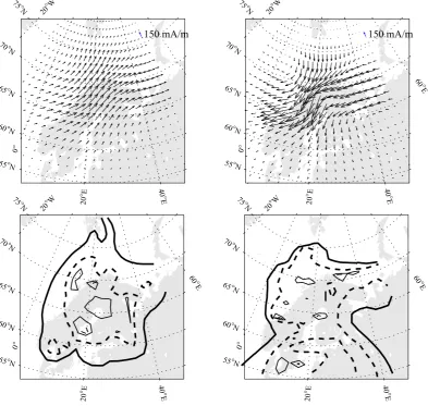
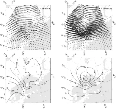
Fig. 3(a). Magnitudes of elementary systems solved for the Omega band using the BEAR array as the ground observation network model. The left panel shows the magnitude of the internal elementary systems, the panel on the right shows the magnitude of the external elementary systems. Dark color denotes positive values. Circles show the magnitude of the standard deviation of each element multiplied by a scale factor ten.
150 mA/m 150 mA/m
20° W
0°
20
°E 40°
E
55°N
60°N
65°
N
70° N
75
°N
20° W
0 °
20
°E 40°
E 60
°E
55°N
60°N
65°
N
70° N
75
°N
20° W
0 °
20
°E 40°
E 60
°E
55°N
60°
N
65°
N
70° N
75
°N
20° W
0°
20
°E 40°
E 60
°E
55°N
60°N
65°
N
70° N
75
°N
-100
-100
-50
-50
-50 0
50
50
50
100
100
150 -300
-200
-200 -100
-100 -100
0
0 100
100 200 100
200
20° W
0°
20
°E 40°
E
55°N
60°
N
65°
N
70° N
75
°N
20° W
0°
20
°E 40°
E 60
°E
55°N
60°
N
65°
N
70° N
75
°N
20° W
0 °
20
°E 40°
E 60
°E
55°N
60°
N
65°
N
70° N
75
°N
20°W
0°
20
°E 40°
E 60
°E
55°N
60°N
65°
N
70° N
75
°N
Fig. 3(c). Same as in Fig. 3(b) but for vertical field (in nT).
a larger number of rejected basis vectors and in general a smoother solution for I. If theσi:s are known, SVD also
yields a statistical estimation for the standard deviations of the fitted parameters inI.
Advantages of the SECS method compared to traditional methods are: 1) We are allowed to choose freely the locations of the elementary systems. So it is possible to make the grid of elementary systems denser at the locations from which we have more magnetic data, i.e. carry out the field separation with a higher spectral resolution at these regions. 2) After the set of elementary systems is chosen and the SVD of the model matrixTis carried out, the I:s andI˜:s in Eq. (7) are obtained for each time step by a single matrix multiplication. This makes the method computationally extremely fast. 3) The mathematical form of the basis functions is very simple. Consequently, evaluation of the model matrixTand the field is computationally efficient. This feature can be utilized for example when using the method in the interpolation of the magnetic field. 4) We knowa pr i or i that the currents causing largest contribution to the ground magnetic field are located in a concentrated sheet in the ionosphere. Thus, by placing the external layer of elementary systems in the approximate location of the ionosphere, we obtain directly information about the currents in this region. 5) We need only divergence-free basis functions, reducing the degree of
freedom by factor 2 compared to modeling a general vector field.
3.
Application of the Method to BEAR and IMAGE
Magnetometer Arrays
In this section the new method is validated for applica-tion with BEAR and IMAGE arrays and is applied to the
magnetic data obtained from the BEAR project. BEAR
20° W
0°
20
°E 40°
E 60
°E
55°N
60°N
65°
N
70° N
75
°N
20° W
0°
20
°E 40°
E
55°N
60°N
65°
N
70° N
75
°N
60
°E
20°W
0°
20
°E 40°
E 60
°E
55°N
60°
N
65°
N
70° N
75
°N
20° W
0°
20
°E 40°
E 60
°E
55°N
60°
N
65°
N
70° N
75
°N
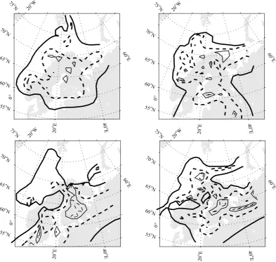
Fig. 4. Top panels: relative error made in the determination of the internal (left panel) and external (right panel) horizontal field using the IMAGE array as the ground observatory network model. Bottom panels: relative error made in the determination of the internal (left panel) and external (right panel) vertical field. Contours are 90 (thick line), 30 (thick dashed line), 10 (thin line) and 5 (thin dashed line) %.
(Fig. 1). Hence it is worthwhile to investigate also the appli-cability of IMAGE to the full field separation with the SECS method.
3.1 Validation of the method for application with BEAR
and IMAGE arrays using synthetic data
First, the performance of the method is tested with syn-thetic data obtained from different ionospheric current mod-els. This is made in similar fashion to Pulkkinen et al.
(2002a) except that in addition to just ionospheric currents, also currents within the Earth are introduced. The procedure is as follows:
1) We use three different, experimentally validated, 3D (both horizontal and field aligned currents included) ionospheric current models: an eastward electrojet having a Gaussian transverse current density distribution, a westward travel-ing surge (WTS) (Amm, 1995) and an Omega band (Amm, 1996). Currents are placed to the height of 110 km.
2) Models are continued outside the initial model area in such a way that the divergence-free condition of the currents (∇ · ji ono = 0) is fulfilled everywhere in the ionospheric
plane.
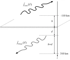
3) We use image currents of the ionospheric currents to mimic the response of the perfectly conducting Earth at a
100 km depth. See Fig. 2.
4) The magnetic field raising from both, ionospheric and im-age sources is computed by Biot-Savart law at ground sta-tions.
5) The computed field at ground stations is put into the SECS method and magnitudes of the elementary systems are solved.
6) The magnetic field is computed back using the solved el-ementary systems and the initial and the fitted magnetic field components are compared.
20° W
0°
20°Ε
40°Ε
60°Ε
55°Ν 60°Ν 65°Ν 70°Ν 75
°N
50%
Fig. 5. The relative error between the measured and modeled north-component of the total variation field when one station at the time is left out in solving SECS’s. Event occurring on June 26, 1998 was used in the test. See text for details.
be carried out. However, the majority of the ground cur-rents flow below 30 km and due to∼100 km spacing of the magnetometer stations, setting the ground layer closer to the surface is not reasonable. Secondly, the decay length of the magnetic field of the elementary system when moving away from the pole of the system should be taken into account. It causes that by setting the spacings of elementary systems much larger than the ones used here, one may end up in a situation where the field observed at one station needs to be explained almost completely by a single elementary system, which of course is not desirable. In addition, by using too large spacings, one may introduce artificial oscillations of the magnetic field between the stations. Because the decay of the field becomes steeper with decreasing radial distance from the element, these effects become larger, i.e. smaller spacings are required when setting the layer closer to the sur-face of the Earth. This is the reason why the ground layer was left to the 30 km depth in this study. By testing the opti-mal trade-off between the resolution and stability, we choose to set singular values being 7% and smaller compared to the largest value to zero in the least-squares solution by SVD. Standard deviations of the magnetic field measurement er-rors are assumed to be 0.1 nT.
To avoid an excessive number of images, results of the tests are shown only for the Omega band case (Figs. 3(a)–
3(c)). For a more illustrative view, we compute
jeq =
2 μ0
n× BH (14)
wherenis a unit vector pointing toward (away from) the cen-ter of the Earth and BH is the horizontal magnetic field. The
vectors jeq represent the equivalent currents immediately
above (below) the ground, i.e. external (internal) source. Note that equivalent currents computed this way are not ex-act in spherical geometry (e.g., Pulkkinenet al., 2002a). By relative accuracy (or error) we mean in the discussion below the percentage of the difference between the model field and true field from the true field, i.e. 100·|(Bmodel−Btr ue)/Btr ue|,
where in the case of the horizontal field,B= | BH|.
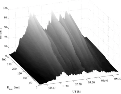
Fig. 6. Rms error of the fit between the modeled and measured ground magnetic field when the height of the ionospheric SECS layer is varied from 0 to 300 km. The ground layer is fixed at the depth of 30 km. Test is made for the June 26, 1998 event.
the relative errors between the initial and solved magnetic fields are shown. It is seen that the basic shape of the both internal and external field is captured well by SECS’s, largest deviations are found at the outer edges of the SECS grids, as expected since these are the regions from which we have least information. In contrast to results in Pulkkinenet al.
(2002a), now Svalbard (northernmost part of the BEAR ar-ray) and the area between Svalbard and continent is poorly modeled, emphasizing the need of a dense 2D array for a reliable field separation. The relative error for both internal and external field vary from 10 to 30% at the area of the main BEAR. In the vertical field the error is larger due to smaller spatial scales than in the horizontal field, being less than 30% in very limited region of BEAR.
In the case of the Gaussian current sheet the errors in the solved fields are quite small. The relative error in the total horizontal field for both internal and external parts is less than 30% and in the vertical field less than 10% in the area of the BEAR array. The error in the horizontal field is smaller in the region of the main current flow (northern part of BEAR), being there also less than 10%.
In the case of the WTS, the SECS method becomes less accurate compared to the Omega band and the electrojet case. This is due to smaller spatial scales related to the WTS model. Although the basic shape of the field is modeled relatively well, the relative error in the horizontal field for both internal and external components is as large as 30% also at the region of the main current flow. The corresponding
error in the vertical magnetic field component is, as in the electrojet case, slightly smaller than for the horizontal field, being between 10–30% for both internal and external field at the main BEAR region.
In order to investigate the potential of the sparser IMAGE array tests identical to ones above were carried out. Results for the Omega band are shown in Fig. 4 where now only the relative errors are shown. The field is separated almost equally well to the BEAR array case. Similar results were obtained for Gaussian electrojet too, however, in the WTS case, the relative accuracies better than 30% were centered to even more limited portion of the array than with the BEAR.
The similarity of the test results between the IMAGE and BEAR arrays is partly due to fact that the largest gradients in the model fields are in the vicinity of the denser part of IMAGE which equals the northern BEAR array (see Fig. 1). However, IMAGE is notably sparser from its southern parts and some deviations could be expected. The absence of such deviations indicates that, at least in the case of our test models, the spatial coverage of the magnetometer array is of more importance than its density. This is emphasized, as was discussed above, also by the apparent uselessness of the Svalbard stations in the field separation, where a 1D array was deployed.
00:30 01:00 01:30 02:00 02:30 03:00 03:30 04:00 04:30 05:00 05:30 60
65 70 75 80 85 90 95
IL
ex
t
/IL
tot
[%]
00:30 01:00 01:30 02:00 02:30 03:00 03:30 04:00 04:30 05:00 05:30
-1200 -1000 -800 -600 -400 -200 0
IL [nT]
UT [h]
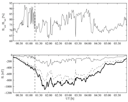
Fig. 7. Top panel: ratio between the external and internal parts of theI L. Bottom panel: external (dashed), internal (thin solid) and the totalI L(thick solid) index computed from the separated magnetic field. The dashed line indicates the time 01:18 UT (compare to Fig. 8).
(4)–(6) to a constant value. Then the field will always be half external, half internal which is obviously not physical. Thus, for example plane wave sources cannot be easily separated.
Summarizing, the general spatial shapes of the separated field components were obtained well by the SECS method. The method was able to separate the field components with the relative error varying from few % up to 30% and worse. The error was depending greatly on the spatial characteristics of the model current: if the spatial scales of the model are smaller than the spacing of the magnetometers, it is impossi-ble to reproduce the detailed structure of the separated field correctly. The error in the modeled field increased rapidly when moving outside the region of the magnetometer array. In addition, when the spatial scales of the field to be sep-arated exceed the extent of the array used field separation cannot be carried out.
3.2 Application of the method to BEAR data and some
characteristics of the separated magneticfield com-ponents during the BEAR period
The field separation was carried out for the entire BEAR one minute database. One common magnetic baseline for the entire array for each day was selected visually to determine the disturbance magnetic field. The set-up of the elementary systems and numerical procedures were identical to the ones used in the test cases.
In Fig. 5 we show the relative error between the mea-sured and the modeled north-component of the magnetic field when one station at the time is left out in deriving
SECS’s. The purpose of the test is to evaluate the interpo-lation capability of the method. Note that divergence-free condition of the magnetic field is always conserved. The rel-ative error is defined here as the median of 100· |Bmeas(ti)− Bmodel(ti)|/|Bmeas(ti)|. Test is made using the most active
period of the entire BEAR project, which was 00:00–10:00 UT June 26, 1998. In the core of the BEAR array the error varies from few % to about 30%, whereas in the northern and southern parts we end up with having errors of about 100%. One should note that at the locations (for example between continent and Svalbard) where the field is initially quite small, large errors are exaggerated due to division by small number in our definition of error. Although not shown here, essentially the same features as for the north-component case are observed also for east- and vertical-components of the magnetic field. In general, it may be concluded that the field interpolated in the central part of BEAR is reliable, at the edges and at the regions where the two-dimensionality of the array is lost, errors may become larger.
20°
100 mA/m 100 mA/m
20°
Fig. 8. Top panels: equivalent current distributions of a possible Omega band event occurring on June 26, 1998 at 01:18 UT. Left panel shows the equivalent currents by internal currents, panel on the right shows the equivalent currents by external currents. Equivalent currents are computed right below (internal) and above (external) the ground. Bottom panels: same as in top panels but for vertical field (in nT).
equally good fit independent of the height of the ionospheric layer of SECS. During 00:45–04:30 UT, the rms error starts to increase roughly above 100 km height, indicative of con-tinuing above the actual source. According to the potential theory, field cannot be continued above the source and that is why we selected the 100 km height for the ionospheric SECS layer. The height dependent dynamics of the iono-spheric currents is also evident in the figure.
To investigate the effect of the induction in the estimation of the I L, the local variant of the global activity index AL
(Kallioet al., 2000), we compute theI Lboth from internal and external parts separately. From Fig. 7 where both parts and the total I L are shown for the June 26, 1998 event, it is seen that on average 80% of theI L is of external origin. At the onset of the event, between 01:30–02:15 UT, up to 30 to 40% of the I L is of internal origin. This is in good ac-cordance with Tanskanenet al.(2001). However, one should note that the variance of the ratio between the external and internal components is quite large throughout the event. One should also note that at the beginning of the event, 00:00– 00:45 UT, and at the end of the event, 04:30–06:00 UT, the internal component of the field is quite large, approximately 30%, indicating imperfect separation caused by too uniform
external source, as was discussed in Subsection 3.1.
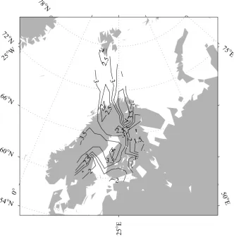
In Fig. 8 snapshots of the internal and external magnetic field are shown for the time 01:18 UT of the June 26, 1998 event. As in the test cases, the horizontal magnetic field vectors are rotated 90 degrees clockwise (anti-clockwise) and are multiplied by 2/μ0 so that the vectors represent the
equivalent currents immediately above (below) the ground. From the external field, patterns corresponding to an Omega band event are seen (compare to Figs. 3(b) and 3(c)). How-ever, the internal field is quite distinct from the test case where just image currents of the source were used. This is to be expected due to complications caused by the 3D conduc-tivity structure of the Earth and by the complex behavior of the source currents. Some of the small scale features in the internal part of the field may also be explained by the fact that, as was discussed in Subsection 3.1, the locations of the poles of the elementary systems is such that it causes larger uncertainty to the internal part of the field.
1.5
2 2
2
2
2
2.5
2.5
2.5 2.5
2.5
3
3
3 3
3
3 3.5
3.5
3.5
4
4 25°W
0°
25
°E
50
°E 75
°E
54°N 60°
N
66° N 72
°N
78
°N
Fig. 9. Logarithm of the integrated conductivity (units in S/m) from the surface to the 60 km depth (i.e. S-map) using regional conductivity models from the BEAR area.
of the region produced by Korjaet al.(2002) (see also, En-gels et al., 2002) by combining separate regional conduc-tivity structure investigations. When comparing the S-map with the internal field in Fig. 8, one can see that in the cen-tral Fennoscandia where the most intense internal horizontal field is obtained, there is a conductivity enhancement giving rise to the induced currents in the region. On the other hand, in the northern part there is a decrease of the conductivity and accordingly induced currents in this region are also no-tably smaller. These features persist for the whole Omega band type event (approximately 01:14–01:22 UT) and thus the separated field seems to be in accordance with the actual conductivity structure of the BEAR region, indicative of a successful separation.
4.
Conclusions
The SECS method, applied earlier to the upward contin-uation of the ground magnetic field, was introduced as a novel approach to the ground variation field separation prob-lem. The characteristics of the method results in several ad-vantages compared to traditional field separation methods. The basic idea of the SECS based separation is to find the least squares solution of the divergence-free elementary cur-rent systems located in two layers, below and above the ground. These layers correspond to external and internal source currents causing the measured total magnetic field on the ground. In theory, any magnetic field can be expressed in
terms of the elementary systems.
The method was tested by using synthetic ionospheric cur-rent models and their image curcur-rent systems placed inside the Earth. These tests proved that the method is applicable to field separation when relatively dense BEAR or IMAGE magnetometer arrays are used. Depending on the source characteristics, namely spatial scales of the source, separated fields were obtained with error varying from few % up to 30%. These tests naturally hold true also for other magne-tometer arrays with similar properties to BEAR and IMAGE. Application of the method to BEAR geomagnetic data also provided reasonable results. Investigation of the induc-tion effects in the local variant of the AL index, I L index, were in accordance with earlier studies and source structures known from previous ionospheric studies where obtained. Comparisons with conductivity maps of the BEAR region supported the results of the field separation. In addition, the method proved to be applicable to interpolation where the physical properties of the magnetic field are conserved. However, it is clear that certain amount of care should al-ways be practiced when carrying out the field separation. For example, the limited coverage of the used array and too uniform source structures cause severe complications to the separation problem and may result in highly unreliable sep-arated fields.
was supported by the Academy of Finland. BEAR is partly funded by INTAS (project 97-1162). IMAGE magnetometer array is an in-ternational project headed by the Finnish Meteorological Institute (http://www.geo.fmi.fi/image). Antti Pulkkinen wishes to thank GEODYNAMO for providing “force” during the prepara-tion of the manuscript. The authors wish to thank Alexei Kuvshinov and another referee for their valuable comments on the manuscript.
Appendix A.
Here we give a simple example on the usage of the terms in Eq. (7) with formulas in Amm and Viljanen (1999). We construct the magnetic field from two elementary systems, one below the ground at (RG, θ1 = 0, φ1 = 0,RG < Re),
whereer andeϑare the radial and polar unit vectors,
respec-tively. From Eq. (A.1) one can easily evaluate the magnetic field produced by these two elementary systems at any point within the shell RG <r < RI. Note that in practice when
elementary systems are distributed on the sphere, vector rota-tions between systems having poles at different(θj, φj)and
(θ˜j,φ˜j)have to be done in order to obtain geometric factors
in a common coordinate system.
References
Amm, O., Direct determination of the local ionospheric Hall conductance distribution from two-dimensional electric and magnetic field data: Ap-plication of the method using models of typical ionospheric situations,J. Geophys. Res.,100, 21473–21488, 1995.
Amm, O., Improved electrodynamic modeling of an omega band and anal-ysis of its current system,J. Geophys. Res.,101, 2677–2684, 1996. Amm, O., Ionospheric elementary current systems in spherical coordinates
and their application,J. Geomag. Geoelectr.,49, 947–955, 1997. Amm, O. and A. Viljanen, Ionospheric disturbance magnetic field
continu-ation from the ground to ionosphere using spherical elementary current systems,Earth Planets Space,51, 431–440, 1999.
Baldwin, R. and H. Frey, Magsat crustal anomalies for Africa: Dawn and dusk data differences and a combined data set,Phys. Earth Planet. Int., 67, 237–250, 1991.
Berdichevsky, M. and M. Zhdanov,Advanced theory of deep geomagnetic sounding,Elsevier Science Publishers B.V., Netherlands, 408 pp., 1984. Chapman, S. and J. Bartels,Geomagnetism,Vol. 2, Clarendon Press,
Ox-ford, 1049 pp., 1940.
Egbert, G., Processing and interpretation of electromagnetic induction array data,Surv. Geophys.,23, 207–249, 2002.
Engels, M., T. Korja, and BEAR Working Group, Multisheet modelling of the electrical conductivity structure in the Fennoscandian Shield,Earth Planets Space,54, 559–573, 2002.
Faynberg, E. B., Separation of the geomagnetic field into a normal and an anomalous part,Geomagn. Aeron.,15, 117–121, 1975.
Golovkov, V. P. and T. I. Zvereva, Separation of the magnetic field into external and internal parts at the surface of prolate spheroid,Geomagn. Aeron.,34, 851–854, 1995.
Haines, G. V., Spherical cap harmonic analysis,J. Geophys. Res.,90, 2583– 2591, 1985.
H¨akkinen, L., T. I. Pulkkinen, H. Nevanlinna, R. Pirjola, and E. Tanskanen, Effects of induced currents on Dst and on magnetic variations at mid-latitude stations,J. Geophys. Res.,107, SMP 7-1–SMP 7-8, 2002. Kallio, E., T. I. Pulkkinen, H. E. J. Koskinen, and A. Viljanen,
Loading-unloading processes in the nightside ionosphere,J. Geophys. Res.,27, 1627–1630, 2000.
Korja, T., M. Engels, A. A. Zhamaletdinov, A. A. Kovtun, N. A. Palshin, M. Yu. Smirnov, A. Tokarev, V. E. Asming, L. L. Vanyan, I. L. Vardaniants, and the BEAR Working Group, Crustal conductivity in Fennoscandia—a compilation of a database on crustal conductance in the Fennoscandian Shield,Earth Planets Space,54, 535–558, 2002.
Langel, R. A., Global magnetic anomaly maps derived from POGO space-craft data,Phys. Earth Planet. Int.,62, 208–230, 1990.
Langel, R. A., The use of low altitude satellite data bases for modeling of core and crustal fields and the separation of external and internal fields,
Surveys in Geophysics,14, 31–87, 1993.
Mersmann, U., W. Baumjohann, F. K¨uppers, and K. Lange, Analysis of an eastward electrojet by means of upward continuation of ground-based magnetometer data,J. Geophys.,45, 281–298, 1979.
Press, W. H., S. A. Teukolsky, W. T. Vetterling, and B. P. Flannery, Nu-merical recipes in FORTRAN: the art of scientific computing,2nd ed., Cambridge University Press, Cambridge, 1992.
Pulkkinen, A., O. Amm, A. Viljanen, and BEAR Working Group, Iono-spheric equivalent current distributions determined with the method of spherical elementary current systems,J. Geophys. Res., 2002a (accepted). Pulkkinen, A., A. Thomson, E. Clarke, and A. McKay, April 2000 geo-magnetic storm: ionospheric drivers of large geogeo-magnetically induced currents,Annales Geophysicae, 2002b (accepted).
Richmond, A. D. and W. Baumjohann, Three-dimensional analysis of mag-netometer array data,J. Geophys.,54, 138–156, 1983.
Rubin, Yu. R., Separation of the variations of the Earth’s magnetic field into parts corresponding to external and internal sources by a sliding smoothing filter,Geomagn. Aeron.,28, 294–296, 1988.
Siebert, M. and W. Kertz, Zur Zerlegung eines lokalen erdmagnetischen Feldes in ¨ausseren und inneren Anteil,Nachr. Akad. Wiss. G¨ottingen, Math.-Phys. Kl. Act. IIa: 87 - 112, 1957.
Tanskanen, E. I., A. Viljanen, T. I. Pulkkinen, R. Pirjola, L. H¨akkinen, A. Pulkkinen, and O. Amm, At substorm onset, 40% of AL comes from underground,J. Geophys. Res.,106, 13119–13134, 2001.
Untiedt, J. and W. Baumjohann, Studies of polar current systems using the IMS Scandinavian magnetometer array,Space Sci. Rev.,63, 245–390, 1993.
Weaver, J. T., On the separation of Local Geomagnetic Fields into External and Internal Parts,Zeitschrift f¨ur Geophysik,30, 29–36, 1964. Weaver, J. T.,Mathematical Methods for Geo-electromagnetic Induction,
Research Studies Press Ltd., England, 316 pp., 1994.
Viljanen, A., K. Kauristie, and K. Pajunp¨a¨a, On induction effects at EISCAT and IMAGE magnetometer stations, Geophys. J. Int., 121, 893–906, 1995.