The irregular variations of the external geomagnetic field
from Intermagnet data
Eric Bellanger, Fatma Anad, Jean-Louis Le Mou¨el, and Mioara Mandea
Laboratoire de g´eomagn´etisme, Institut de Physique du Globe de Paris, 4, place Jussieu, 75252 Paris Cedex 05, France
(Received April 15, 2002; Revised March 28, 2003; Accepted March 31, 2003)
The INTERMAGNETprogram publishes each year aCD-ROMcontaining homogeneous series from a number of magnetic observatories (76 in 1999). These series are definitive one-minute values of the three components of the geomagnetic field. We transform these series using a simple nonlinear analysis tool able to characterize the activity of a signal, and we obtain a remarkably simple activity field, whose space and time variables separate over a large part of the Earth. The time function is almost identical for all observatories, and might be interpreted as an activity index. The—almost stationary—field geometry exhibits a dipole-like structure everywhere except in high latitudes. Key words:Geomagnetic field, irregular variations, INTERMAGNET, absolute derivative.
1.
Introduction
The geomagnetic field results from the superposition of an internal component (the main field and the crustal field) and an external component. The external geomagnetic field varies both in space and time; its geometry is quite compli-cated and its time constants range from sub-milliseconds to decade. The INTERMAGNETprogram publishes each year aCD-ROM containing the minute values of the components of the magnetic field recorded in some 80 observatories. We use these minute values, which allow us to monitor global short time scales phenomena, following the lines of a former paper (Bellangeret al., 2002) devoted to longer time scales (daily averages were used); we process them with a simple nonlinear tool to see whether a simple structure, in space and time, can be extracted from this large dataset, as was the case using daily values.
2.
The Data
All modern magnetic observatories use standard instru-mentation to produce standard data products. Fundamental measurements are one-minute values of the vector compo-nents and of the scalar intensity of the field. The INTER -MAGNETprogram calls for the world’s magnetic observato-ries to be equipped with fluxgate and proton magnetometers (with a resolution of 0.1 nT) operating automatically under computer control. The number of observatories participat-ing in this program has continuously increased, from 41 in 1991 to 76 in 1999. The INTERMAGNET CD-ROMonly con-tains data from participating observatories. These data are definitive one-minute values (data which have been corrected for baseline variations and which have had spikes removed and gaps filled where possible), with an absolute accuracy of ±5 nT, of the three field components: horizontal north-ward (X), horizontal eastnorth-ward (Y) and vertical downnorth-ward (Z). For a full description see the INTERMAGNET Techni-cal Manual (Trigg and Coles, 1999) and the INTERMAGNET web site (http://www.intermagnet.org). For ob-servatory practice, see Jankowski and Sucksdorff (1996).
In this study we use a set of 30 INTERMAGNET obser-vatories providing a reasonably homogeneous distribution of measurements at the Earth’s surface, for the 1996–1997 time-period. The distribution of the observatories, with their IAGA code, is given in Fig. 9. Moreover, a six-year series for the Chambon-la-Forˆet observatory has been analyzed.
3.
The Absolute Derivative
We have 3 × M series Xm(tn), Ym(tn), Zm(tn), m = 1,2. . .M;Mis the number of observatories;tnis time, reck-oned in minutes; the range spanned bynis different for each observatory. Let F(t)be one of these time-series and con-sider the first differenceF(t). We will callF(t)derivative; but we do not look for a better estimate of the time deriva-tive, by using for example classical several points formulae; in fact, we are considering ranges (variations of the consid-ered function over the considconsid-ered minute). The absolute first difference|F(t)|is
|F(t)| = |F(t+1)−F(t)|, (1)
and the average of |F(t)| over a sliding time window of lengthT (Blanteret al., submitted) is
|F(t)|T = contributions of local time components of the magnetic field caused by partial ring currents and magnetotail currents, as well as the contribution of Sq, are then largely attenuated in our 24-hour averages.
Mathematically, the average absolute derivative is the total variation of the (sampled) function over an interval of length T (c.f. Riemann-Stieltjes integrals). The variation measures the “up-and-down” distance traced out by the “point” F(t) ast moves in the considered interval. It is used here to
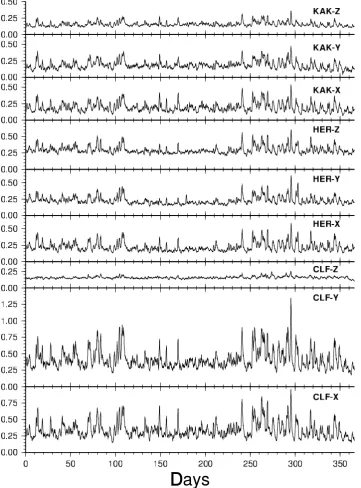
Fig. 1. Averaged absolute derivative of the three components of the magnetic field in CLF, HER and KAK observatories for year 1996 (units are nT/min).
acterize the “activity” of the function: computed from geo-magnetic series, the average absolute derivative has higher levels during disturbed days than during quiet days. Since we compute the average absolute derivative for each compo-nent of the magnetic field, we obtain a new field which we call an activity field (see below).
4.
Results
Some of the results are illustrated in Fig. 1. The graphs represent|X|T,|Y|T, and|Z|T as computed following (2) in different observatories.
It is remarkable to notice how the|X|T,|Y|T, and|Z|T curves look alike in a given observatory, but also how all the curves, for almost all observatories, look similar, even in tiny details. Figure 2 gives an enlarged representation
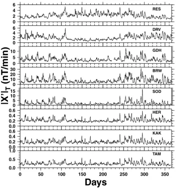
of eight |X|T curves corresponding to Tamanrasset (TAM), Kakioka (KAK), Hermanus (HER), Sodankyl¨a (SOD), Barrow (BAR), Godhavn (GDH), Dumont d’Urville (DRV) and Reso-lute Bay (RES); these observatories are located respectively in Algeria, Japan, South Africa, Finland, Alaska, Greenland, Antarctica and Canada.
These observatories cover a wide range of corrected ge-omagnetic latitudes, from equatorial regions (TAM) to polar caps (DRVandRES). Except for polar cap observatories, all
0.0
Fig. 2. |X|T in TAM, KAK, HER, SOD, BRW, GDH, DRV and RES for year 1996. The corrected geomagnetic latitudes of these observatories are
respectively 9◦, 26◦,−43◦, 64◦, 70◦, 76◦,−81◦and 84◦.
in the reference level with an opposite phase between north pole and south pole), and has difficulty to quickly recover its reference level after strong activity peaks.
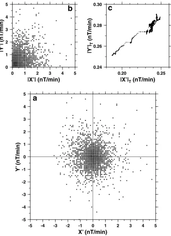
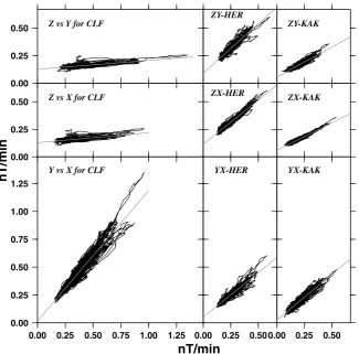
The averaging overT clearly shows the global structure: Figure 3 displays three “phase diagrams”, (X(t), Y(t)), (|X(t)|, |Y(t)|) and (|X|T, |Y|T) for two disturbed days inCLF. No polarization can be derived from the first two diagrams, whereas a clear linear polarization appears when a 1-day averaging of the absolute derivatives is performed. The linear polarization is conserved when considering two years of data (1996–1997), and the correlation coefficients between different components in a given observatory are bet-ter than 0.90 (Fig. 4). Despite the quite different behav-ior between polar cap observatories and lower latitude ones, the polarization in polar cap observatories is as strong (see Fig. 5) as in lower latitude ones, and the correlation coeffi-cients are large (the correlation coefficient between|X|Tand |Y|T is 0.95 forRES, and 0.97 forDRV).
To get an estimate of the correlation between series from different observatories, we draw polarization diagrams and compute the corresponding cross-correlation values. For ex-ample, considering|X|T inCLFand|X|T inKAK(Fig. 6), the correlation coefficient is 0.93.
A strong advantage of using the absolute derivative (or
first difference) from one-minute values is that it practically does not rely on the absolute values of the magnetic measure-ments,i.e.on good baselines. A slow drift of these baselines will have a small but negligible effect on|F(t)|and|F(t)|T. As for the short-term behavior of baselines, it is rather easy to control it; furthermore, the baselines have been carefully examined when submitted to the INTERMAGNET CD-ROM committee.
5.
The Reference Level and UT Dependence
Let us recall that transient variations of the external ge-omagnetic field are classified as regular and irregular vari-ations (Mayaud, 1978); the former are due to permanent sources of field which cause the regular occurrence, every day, of a certain variation during certain local times at a given point on the Earth; the latter are generated by sources which do not permanently exist, which makes their occurrence ir-regular.Let us write,
Be(r,t)=SR(r,t)+DI(r,t) , (3)
-5 -4 -3 -2 -1 0 1 2 3 4 5
Y’
(nT/min)
-5 -4 -3 -2 -1 0 1 2 3 4 5
X’ (nT/min)
a
0 1 2 3 4 5
|Y’| (nT/min)
0 1 2 3 4 5
|X’| (nT/min)
b
0.24 0.26 0.28 0.30
|Y’|
T
(nT/min)
0.20 0.25
|X’|
T(nT/min)
c
Fig. 3. Phase diagrams in CLF for January 13th and 14th, 1996 (perturbed days). a)YvsX;b)|Y|vs|X|andc)|Y|Tvs|X|T(units are nT/min).
Note that 3 days are used to compute these two days of average absolute derivative, see Eq. (2).
DI in Section 7. A drawback of using an absolute deriva-tive as (1) or (2) is that, the additivity property being lost, it is not so easy to separate the contributions of the two com-ponents of (3). Let us look at some orders of magnitude. SR is supposed regular; It cannot give rise to variations of 50 nT in less than 3 hours. Its contribution to|F(t)|is then smaller than 0.28 nT/min. As for the measurement error, it comes from Section 2 that its contribution to the differ-ences |F(t +1)− F(t)| and|F(t)|T can be estimated to 0.1×√2 =0.14 nT/min. It can then be supposed that the value of|F(t)|T, in the case of a nullDIfield (over a day) is of the order of 0.32 nT/min. Looking at the graphs of Fig. 1, it appears that in most stations the reference level (defined as the lower envelope of the curves) has a value of this order of magnitude (in fact, in most cases, lesser).
ob-0.00 0.25 0.50 0.75 1.00 1.25
nT/min
0.00 0.25 0.50 0.75 1.00 1.25
nT/min
Y vs X for CLF
0.00 0.25
0.50 Z vs X for CLF 0.00
0.25
0.50 Z vs Y for CLF
0.00 0.25 0.50
YX-HER ZX-HER ZY-HER
0.00 0.25 0.50
YX-KAK ZX-KAK ZY-KAK
Fig. 4. Polarization diagrams in CLF, HER and KAK observatories for years 1996 and 1997.
0 1 2 3 4 5
|Y’|
T
(nT/min) in RES
0 1 2 3 4 5 6
|X’|T (nT/min) in RES
Fig. 5. Polarization diagram|Y|Tvs|X|Tin RES for year 1996. The correlation coefficient is 0.95.
0.0 0.2 0.4 0.6
|X’|
T
(nT/min) in KAK
0.0 0.2 0.4 0.6 0.8 1.0
|X’|T (nT/min) in CLF
0.75 0.80 0.85 0.90 0.95 1.00
Cr
oss-correlation C(
θ
)
-10 -8 -6 -4 -2 0 2 4 6 8 10
Lag
θ
(hours)
Fig. 7. Correlation coefficientsc(θ)for the year 1996: solid line between|X(t)|Tin Kakioka and|X(t+θ)|Tin Chambon-la-Forˆet; dashed-dotted line
between Kakioka and Hermanus; dashed line between Chambon-la-Forˆet and Hermanus.
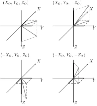
Fig. 8. Different possible directions forωωω(O)at an observatoryO; (XO,
YO,ZO) corresponding toDO,IO; (XO,YO,−ZO) toDO,−IO; (−XO,
YO,ZO) to(π−DO),IO and (−XO,YO,−ZO) to(π−DO),−IO.
Four other possible orientations can be obtained by changingYOto−YO.
served variations do not depend on local time.
6.
The Field
(P,t)Let us denote(P,t)a field whose absolute values of the components are respectively |X|T(P,t), |Y|T(P,t) and |Z|T(P,t), wherePis position. As we considered absolute values, we are not able, at this stage, to recover the signs of the components, see below. (P,t)is derived from DI as stated above. Since at each observatory, for each component (in a first but good approximation), the temporal variations are similar, it follows that, at the same approximation, the time and space variations of(P,t)separate:
(P,t)=ωωω(P)R(t) . (4)
R(t)is taken positive (an activity function),ωωω(P) charac-terizes the geometry of the irregular variations processed as indicated.
6.1 Geometry
In Bellangeret al.(2002), we made a (rather qualitative) analysis of the fieldωωω(P)in the case of daily means, and showed that it was axially symmetrical around an axis whose colatitude and longitude were (14±3 ;−82±10) degrees. Things appear less simple here. It should be said that(P,t) is a rather special field (an activity field, as already said, which cannot be analyzed as straightforwardly as classical fields). We just present here a first step to the analysis of
ωωω(P).
At each point P we compute the direction of ωωω(P) in the following way: we determine the declination D (and in a similar way the inclination I) ofωωω by computing the regression line of the graphs representing|Y|T versus|X|T (Fig. 4); denoting(|Y|T/|X|T)exthe slope of the regression line,Dis taken as
D=tan−1(|Y|T/|X|T)ex
. (5)
Nine examples of regression computation are shown on Fig. 4. The error on the estimates of the slopes is small enough for the precision being better than 3 degrees in D andI. These estimates are free from the value of the refer-ence level as defined in Section 5,i.e.of the intercepts of the regression lines with thexandyaxes.
We also estimate the length of the horizontal component ofωωω,ωωω⊥, in the following way:
ωωω⊥ =
|X|T2+ |Y|T2, (6)
val-225° 270° 315° 0° 45° 90° 135° 180°
Fig. 9. Map of the horizontal componentωωω⊥ofωωω. IAGA observatory codes are used.Black arrows:we have takenXandY, the components ofωωω⊥, positive in every observatory (but symmetric orientations with respect toO xorO yaxes are possible from the analysis at an individual station; see text).
Gray arrows:a more likely direction for the activity field in some observatories, if we assume that the fieldωωωhas a dipolar geometry; with this choice
the lower latitude activity field present an axial geometry around the axis defined by (θ0=30◦;φ0= −80◦).
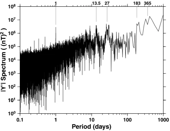
Fig. 10. Energy spectrum for 6 years of absolute minute differences of the East component of the magnetic field (|Y|) in CLF.
ues forDand two forI(Fig. 8). In fact, the number of com-binations is reduced from eight to four, since there is no need to distinguish betweenωωωand−ωωω(is a transient field). In Bellangeret al.(2002) we used simple regularity conditions to discriminate between the four possible situations at each observatory, and then to construct a physical variation field: theXcomponent ofωωωwas taken positive everywhere and the sign of theY and Z components at each observatory were chosen such asωωωvectors from nearby observatories pointed closely in the same direction (no erratic variation ofωωω(P)) and assuming that the fieldωωω(P)had rather a dipolar geom-etry (to start with the simplest). The situation is less simple here. We show, on the map of Fig. 9, the length of the hor-izontal componentωωω⊥ ofωωω, and the direction obtained by taking systematically bothX andY, the components ofωωω⊥,
positive (symmetric orientations with respect to O x or O y axes are possible when analyzing data for an individual sta-tion).
0.0
uto correlation C
Y*
(see Fig. 9) and we found that the lower latitude activity field might present an axial geometry around the axis defined by (θ0 = 30◦ ;φ0 = −80◦). The dipole-like geometry of the
activity field obtained from one-minute values is, however, less obvious than the one derived from daily means, and the inferred axis is quite different from the Gauss dipole of the internal main field. Let us stress that at minute time scales the varying magnetic field is more affected by local induc-tion effects. We will come back to the geometry of the activ-ity field later, after gathering all the available data series; in this respect, methods like the ones developed in Hulotet al. (1997) and Khokhlovet al.(1997) could be used.
6.2 Recurrences.
Let us briefly elaborate on the temporal behavior of our activity field,i.e.functionR(t)in (4). Some kind of average of a number of|X|T,|Y|T, and|Z|T curves could be taken; we will simply consider as representative the curve|Y|T in Chambon-la-Forˆet.
We consider the 6-year long series of|Y(t+1)−Y(t)| = |Y(t)|, without averaging over a day. Figure 10 represents the spectrum of|Y(t)|. Expected peaks can be recovered at 1 day (and harmonics), 27 days (and harmonics), and probably one year and six months, although the length of the series, 6 years, is rather short for revealing such long periods with a simple Fourier transform. These periodicities are well known and we shall not discuss them any further in this paper devoted to short time scales (events shorter than a few days, see Fig. 1) variations of the irregular field. Nevertheless, our array of INTERMAGNETobservatories will allow us to study in a new way the geographical distribution of the intensity of these spectral peaks (Banks, 1969; Achacheet al., 1981; Olsen, 1999).
7.
Discussion, Conclusion and Perspectives
We will not try to give here a full interpretation of our main results, which are the strong resemblance of all the|X|T,|Y|T and|Z|T curves, the polarization of the activity field along a direction independent of the time in all obser-vatories (even including data from polar caps obserobser-vatories), and, possibly, an axial geometry ofωωω⊥(P)for low and mid-dle latitudes observatories, but will only make a few com-ments and point out some perspectives.
At the end of Section 6.1, we emphasized the strong val-ues of ωωω⊥(P) in high latitude observatories. Following Fukushima and Kamide (1973), let us recall the world ge-omagnetic disturbance fieldDIas:
DI=DR+DP+(DCF+DT) , (7)
in whichDRwas thought to be the geomagnetic disturbance field generated by a ring current flowing in the geomagnetic equatorial plane at a geocentric distance of several Earth’s radii. It has been shown, however, that there is not a “ring current”, but rather numerous partial rings that feed field-aligned currents to and from the magnetosphere (Campbell, 1996). DP is the geomagnetic disturbance caused primarily by intense electrojets flowing in the ionosphere of the polar region (including the auroral zone) and their accompanying currents in the ionosphere or magnetosphere, or both. DCF represents disturbance caused by the interaction between the corpuscular flux of the solar plasma stream and the Earth.DT represents disturbance caused by the electric current flowing in the tail of the magnetosphere. DCFandDTcan generally be neglected at the Earth’s surface.
Our observations show thatDPplays an important part in our(P,t)field (high values in high latitudes), and thatDR andDPare intimately correlated (high resemblance between curves from all latitudes), which might be expected if the cor-responding current systems are physically linked (Campbell, 1996).
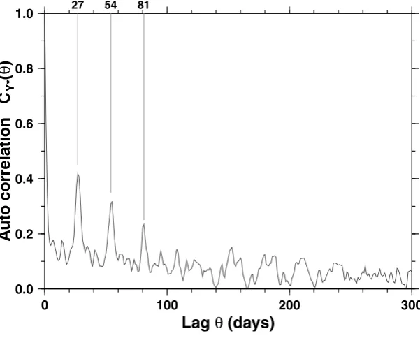
us rather consider the series of daily values
Y∗(k)= |Y(o(k))|T , (8)
timeo(k)being 0h00:01 of dayk. It is clear, from the way it is computed, thatY∗(k)is a good estimate of the activity range of Y for dayk—in fact,Y∗(k)is, from a mathematical point of view, a close estimate of the total variation of Y over dayk. An interesting and timely question is the predictabil-ity of theY∗(k)series, as part of the important problem of space weather forecasting. In this paper, we will simply com-pute the auto-correlation function ofY∗(k)for the six years long series of Chambon-la-Forˆet (2200 data points). Fig-ure 11 represents the auto-correlationCY∗(θ)ofY∗(k). The 27-day periodicity of the activity function clearly appears in CY∗(θ). The second interesting feature is the value of the auto-correlation for a 1-day lag: CY∗(1)= 0.61, which in-dicates persistence. Nevertheless, the auto-correlation drops fast: only 0.35 for a two-day lag, which tends to indicate that long-term prediction is not possible. In a future study (Bel-langeret al., 2003), we will apply methods used in seismol-ogy, like the(η, τ)Molchan (1997) diagram, to the forecast-ing of magnetic activity, usforecast-ing againY∗(k); more precisely, we will assess rigorously the statistical significance of the forecasting. Let us recall thatY∗(k), as demonstrated above, is a representation ofR∗(k)and is of worldwide significance. The same analysis we performed here with 24 hours daily averages of one-minute value absolute first differences can be performed with hourly averages. Subsequent prediction studies will be richer.
Acknowledgments. M. Matsushima, an anonymous referee and Yasuo Ogawa, the editor in charge, made useful suggestions to improve the manuscript. This is IPGP contribution n◦1906.
References
Achache, J., J.-L. Le Mou¨el, and V. Courtillot, Long-period geomagnetic variations and mantle conductivity: an inversion using Bailey’s method,
Geophys. J. R. Astron. Soc.,65, 579–601, 1981.
Banks, R. J., Geomagnetic variations and the electrical conductivity of the upper mantle,Geophys. J. R. Astron. Soc.,17, 457–487, 1969. Bellanger, E., E. M. Blanter, J.-L. Le Mou¨el, M. Mandea, and M. G.
Shnir-man, On the geometry of the external geomagnetic irregular variations,J. Geophys. Res.,107, 10.1029/2001JA900112, 2002.
Bellanger, E., V. G. Kossobokov, and J.-L. Le Mou¨el, Predictability of geomagnetic series,Ann. G´eophys., 2003 (in press).
Blanter, E. M., M. G. Shnirman, and J.-L. Le Mou¨el, Solar activity and variability of geophysical time series; the synchronizing driving force,J. Geophys. Res., 2003 (submitted).
Campbell, W. H.,Dstis not a pure ring-current index,EOS Trans. Amer. Geophys. Union,77(30), 283–285, July 23 1996.
Fukushima, N. and Y. Kamide, Partial ring current models for worldwide ge-omagnetic disturbances,Rev. Geophys. Space Phys.,11, 795–853, 1973. Hulot, G., A. Khokhlov, and J.-L. Le Mou¨el, Uniqueness of mainly dipolar magnetic fields recovered from directional data,Geophys. J. Int.,129, 347–354, 1997.
Jankowski, J. and C. Sucksdorff,Guide for Magnetic Measurements and Observatory Practice, IAGA, 1996.
Khokhlov, A., G. Hulot, and J.-L. Le Mou¨el, On the Backus effect—I,
Geophys. J. Int.,130, 701–703, 1997.
Mayaud, P. N., Morphology of the transient irregular variations of the ter-restrial magnetic field, and their main statistical laws,Ann. G´eophys.,34, 243, 1978.
Molchan, G. M., Earthquake prediction as a decision-making problem,Pure Appl. Geophys.,149, 233–247, 1997.
Olsen, N., Long-period (30 days–1 year) electromagnetic sounding and the electrical conductivity of the lower mantle beneath Europe,Geophys. J. Int.,138, 179–187, 1999.
Trigg, D. F. and R. L. Coles, Intermagnet Technical Reference Manual, 1999.