Emerging Paradigms in Quantum Error Correction and Quantum Cryptography

(1)

Emerging Paradigms in Quantum Error Correction and Quantum

Cryptography

Thesis by

Prabha Mandayam Doddamane

In Partial Fulfillment of the Requirements for the Degree of

Doctor of Philosophy

California Institute of Technology Pasadena, California

2011

(2)

c

2011

(3)

To

(4)

Acknowledgements

As I get ready to submit my doctoral thesis, it is a pleasure to finally acknowledge and thank everyone who has been a part of this incredible journey.

First and foremost, thanks to my adviser Prof. John Preskill for his help and advice these past six years. Being his student and interacting with him has been a rare privilege and a great learning experience for me. Apart from having learnt some of the fundamental concepts of quantum information processing from him, I have also learnt a lot from his approach to scientific research, in particular, the importance of motivating and communicating the physical intuition behind one’s research. But most of all, thank you John, for your patience and understanding during my initial blundering forays into research. And thanks also, for letting me be a part of the great institution that IQI is. With its array of post-docs working in diverse areas, and a continuous stream of visitors, I couldn’t have asked for a better place in which to start my research career in quantum information.

(5)

and mentor that you are. And thanks also, for introducing me to the wonderful world of quantum cryptography! A special word of thanks to Niranjan Balachandran whose expertise in combinatorics and graph theory helped us formalize some of the proofs in Chapter 3.

Thanks to Profs. Alexei Kitaev, Oskar Painter and Gil Refael for serving on my thesis commit-tee. Thanks also to Kovid, Panos, Graeme, Greg, Ersen, Issac, Jeongwan, Robert, Robin, Liang and other colleagues at IQI.

I would also like to acknowledge here, some of the teachers who played a motivational role during my student days in India, especially Prof. Arul Lakshminarayanan and Prof. M.V.Satyanarayana. Arul, with whom I worked on my Masters’ thesis, has been a great friend and guide. MVS, whose fierce passion for physics has inspired many a student, has been an honest critique and a constant well-wisher.

This thesis is dedicated to my parents, for it was with them that this journey really began. Back in high school, it was through my mother Vijayalakshmi that I discovered the joy of doing mathematics. And it was from my father Srinivas, who has been an academic all his life, that I developed an interest in research and teaching. Indeed, my fascination for quantum mechanics dates back to many simulating discussions with my father during my undergraduate days—he is among the best teachers of the subject I have seen to date! I am grateful to my parents, not only for shaping my approach to science, but for the larger lessons that I have had a chance to learn from them, through the values they exude in their everyday lives.

To my sister Nitya, my oldest friend and confidante, thanks for sharing in all the ups and downs of these PhD years. To Uday, Shweta, Sushree, JK, Mansi, Setu, Mayank, Shankar, Varun, Shriharsh, Naresh, Chithra, Arundhati, Sameer, Pinkesh, Vikram, Tejaswi and all my other friends at Caltech, thank you for making this place a home away from home for me. Thank you for all the music, food, concerts, plays and above all, the companionship, which truly enriched my graduate school experience. Thanks also to my friends from India—Jeevisha, Ashok, Devi and Roshni—who have stood by me through thick and thin. I am thankful to my husband’s parents for their keen interest in my progress and their support and encouragement.

(6)

Abstract

We study two novel paradigms in quantum error correction and quantum cryptography—approximate quan-tum error correction andnoisy-storage cryptography—which explore alternate approaches for dealing with quantum noise. Approximate quantum error correction seeks to relax the constraint of perfect error

correc-tion and construct codes that might be better adapted to correct for specific noise models. Noisy-storage

cryptography relies on the power of quantum noise to execute two-party cryptographic tasks securely.

Motivated by examples of approximately correcting codes, which make use of fewer physical resources

than perfect codes and still obtain comparable levels of fidelity, we study the problem of finding and

char-acterizing such codes in general. We construct for the first time a universal, near-optimal recovery map

for approximate quantum error correction (AQEC), with optimality defined in terms of worst-case fidelity.

Using the analytical form of this recovery, we also obtain easily verifiable conditions for AQEC. This in turn

leads to a simple algorithm for identifying good approximate codes, without having to perform a difficult

optimization over all recovery maps for every possible encoding.

Noisy-storage cryptography envisions a setting where two-party cryptographic protocols can be securely

implemented based solely on the assumption that the quantum storage device possessed by either party is

noisy and bounded. Here, we construct two-party protocols (using higher-dimensional states) that are secure

even when a dishonest player can store all but a small fraction of the information transmitted during the

protocol, in his noiseless quantum memory. We also show that when his memory is noisy, security can be

extended to a larger class of noisy quantum memories. Our result demonstrates that the physical limits of

the quantum noisy-storage model are indeed achievable, albeit asymptotically.

We also describe our investigations on obtaining strong entropic uncertainty relations using symmetric

complementary bases. Uncertainty relations are an important and useful resource in analyzing the security

of quantum cryptographic protocols, in addition to being of interest from a foundational standpoint. We

present a novel construction of sets of symmetric, complementary bases in dimension d = 2n

, which are

cyclically permuted under the action of a unitary transformation. We also obtain new lower bounds for

(7)

Chapter 1

Introduction

It has been over two decades since the idea of quantum information processing has captured the imagination of physicists, computer scientists, and information theorists alike. Two important discoveries that provided critical impetus for the growth of the field in its nascent stages have been quantum error correction and quantum cryptography. The discovery of quantum error correcting codes in the mid-nineties [22, 120, 123] demonstrated that it is indeed possible to perform quantum information processing reliably in the presence of noise. The early quantum cryptographic protocols discovered in the pervious decade [11, 13, 42] demonstrated the usefulness of quantum systems in performing fundamentally unbreakable cryptographic tasks.

Na¨ıvely, the problem of quantum error correction appears daunting in the face of several con-ceptual challenges. Theno-cloning theorem[133] rules out the possibility of constructing quantum repetition codes analogous to classical repetition codes. Also, since quantum errors are continuous, it is difficult to measure and identify the errors with precision. Furthermore, since the measurement process actually destroys or modifies quantum information, we cannot directly employ the standard classical technique of observing the output of the channel and selecting the decoding procedure on that basis. However, discovery of necessary and sufficient conditions for quantum error correction in general noise models [15, 43, 70] demonstrated how quantum codes can be constructed in spite of these challenges. On the other hand, for cryptographic protocols, these very properties prove to be useful in achieving security against an eavesdropper.

(11)

tolerance threshold theorem [2, 39, 71, 121], and more recent ideas of dynamical decoupling [63, 126] and subsystem or operator quantum error correction [82]. We refer the reader to [102, 103] for a detailed overview of some of these important developments.

Quantum cryptography has also come a long way since the first quantum key distribution (QKD) protocol. Known as theBB84 protocolin honor of its creators [11], this became a prototype for later quantum cryptographic protocols. Starting from experimental implementations over a distance of 32.5 cm in 1989 [12], today we have experimental setups that have successfully demonstrated QKD over distances of hundreds of kilometers [59, 116]. An alternate view of QKD based on quantum entanglement [42] motivated newer ideas like quantum privacy amplification [35] and made the task of proving the security of QKD protocols much easier. Since then, several security proofs have been constructed [87, 95, 107, 122] leading to stronger QKD protocols that are unconditionally secure against general attacks. However, moving beyond key distribution has proved to be a big challenge in the quantum setting.

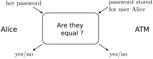
Early results showed that unconditional security was not possible for non-QKD protocols such as quantum bit commitment [33, 96] and quantum oblivious transfer [86]. Bit commitment and oblivious transfer are protocols that help to realize practical two-party functions such as online auctions or secure identification, where the participating parties do not trust each other. We will describe oblivious transfer in Section 4.4 and refer to [127] for a complete introduction to these and other two-party cryptographic tasks. In fact, it was shown in [86] that it is impossible to implement any such two-party quantum cryptographic protocol securely, without imposing some restrictions on the dishonest party.

Quantum cryptography also admits phenomena which do not have a classical analog, like the phenomenon of information locking [38]. The development of quantum cryptography has also spurred tremendous interest in the study of quantum information measures, in particular the prop-erties of R´enyi entropies and extensions thereof [74,109], which lie at the heart of most cryptographic security proofs today.

(12)

of noisy storage cryptography [76, 115] which envisions a setting where two-party cryptographic protocols can be securely implemented based solely on the assumption that the quantum storage device possessed by the adversary is noisy and bounded. In what follows, we introduce and motivate these two ideas in greater detail.

1.1

Adapting to Quantum Noise: Approximate Quantum Error

Correction

We have already referred to some of the important theoretical advances in the theory of quantum error correction (QEC). While the standard paradigm of QEC is well-understood and rests on a solid mathematical foundation, the discovery of approximate codes [46,85] has shown that this standard framework might be somewhat restrictive. Approximate quantum error correction (AQEC) relaxes the constraint of perfect recovery and instead seeks codes that recover the input state with high enough fidelity. A typical quantum error correcting code is designed to perfectly correct only some subset of the errors that constitute the noise channel, in particular the ones that occur with a higher probability. Every perfect code is thus an approximate code for the least probable errors of the channel. These standard codes are, however, designed based on conditions that demand perfect correction of the complete noise channel. The theory of perfect quantum error correction is discussed in some detail in Section 2.1.2.

In practice, experimental setups for creating and storing qubits are usually characterized by a certain dominant noise process. For example, in many setups based on quantum optics, amplitude damping noise [26,49] is most dominant. More recently, it was observed that in some superconduct-ing qubit systems, dephassuperconduct-ing noise is stronger than other noise processes by a factor of 103 _{[1, 3].}

(13)

requirement for perfect QEC—one might be able to encode the same amount of information into fewer qubits while retaining a nearly identical level of protection from the noise.

These observations indicate the importance of developing a general theory of approximate quan-tum error correction. There are two possible approaches to characterize approximate codes. The Leung et al. approximate code was constructed as a simple perturbation of a perfect code, raising the possibility that perturbing the perfect error correction conditions might yield conditions for approximate correction [90]. Alternately, approximate quantum error correction can be formulated as an optimization problem [46,135]. Given a noise channel and the information we need to encode, AQEC is the problem of finding the optimal encoding and recovery maps, with optimality defined in terms of a chosen measure of accuracy of recovery.

In our work presented in Chapter 2, we combine both these aspects of approximate error cor-rection via a universal recovery map, namely thetranspose channel. On the one hand, by defining optimality in terms of the worst-case fidelity, we demonstrate that the transpose channel is a near-optimal recovery map for any noise channel. We also show that the perfect error correcting conditions can be rewritten in terms of the transpose channel. Combining this with our fidelity bound, we are able to write down simple conditions for approximate quantum error correction, which are indeed obtained as perturbations of the perfect QEC conditions. Earlier studies [8] had in fact shown that the transpose channel is a near-optimal recovery for an average fidelity mea-sure based on the entanglement fidelity. Indeed, while the problem of finding optimal codes for the entanglement fidelity has been studied in the recent past [17, 45, 124], we present for the first time an analytical description of a recovery map that is close to optimal for the worst-case fidelity. The worst-case fidelity involves minimizing the fidelity between the input and output states over all input states in contrast to the average fidelity which is simply an average over input states. Optimizing for the worst-case measure thus provides a stronger assurance that all the information in the input space is well protected.

(14)

a fault tolerant quantum computing architecture.

1.2

Using the Power of Quantum Noise: Noisy-Storage

Crypto-graphy

As mentioned above, one of the early negative results in quantum cryptography was the discovery that secure two-party quantum cryptography is not possible without additional assumptions [86]. In the classical setting, the usual assumptions that go into realizing secure two-party protocols involve mathematical hardness results and a restriction on the computing power of a cheating party. An interesting physical assumption that also leads to security in the classical setting is to assume a restriction on the amount of classical storage a cheating party can use [21, 94]. However, in this classical bounded-storage model, the cheating party requires only quadratically more storage than the honest party to break the security. Furthermore, a tight bound on classical storage is not easily enforceable in today’s context. Since storing quantum states for any significant length of time still remains a hard problem, the quantum analog of the classical bounded-storage model might be a more realistic prospect.

In this setting of bounded quantum storage, protocols for secure implementation of quantum bit commitment and oblivious transfer were demonstrated under the assumption that a cheating party cannot store any quantum information at all [14, 29]. Recently, this bound was improved, showing that quantum oblivious transfer can be securely implemented if the cheating party can store no more than a fourth of the qubits transmitted during the protocol [30, 31]. An alternate physical situation to consider is of course the case where the cheating party’s quantum storage is noisy, while allowing for a larger storage size. In this quantum noisy-storage setting, a protocol for secure oblivious transfer was constructed [115,128] with the additional constraint that the cheating party could only perform product measurements on the qubits received during the protocol.

(15)

and the storage rate of the cheating party. When specialized to the case of bounded quantum storage (when the storage is noiseless) these protocols were shown to be secure so long as the cheating party cannot store more than half the qubits transmitted. This is quite an improvement over the earlier bound obtained for the bounded-storage model.

In the bounded storage model, it is intuitively clear that if a cheating party were able to store

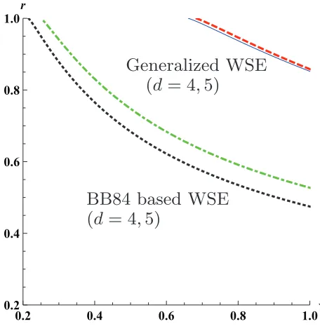
allof the information transmitted during a protocol, security cannot be achieved. This is equivalent to saying that the storage rate must be less than one, if a protocol is to be secure. Conversely, one can ask the question as to whether it is always possible to achieve security if the storage rate is strictly less than unity. The protocols constructed so far do not answer this question conclusively. While the best protocol achieves security so long as the storage rate is less than a half in the bounded-storage model, the question as to whether the physical limit of one is achievable remained unresolved. We address this question in our work presented in Chapter 4, and demonstrate that it is indeed possible to achieve security if the cheating party’s storage rate is strictly less than one. To achieve this physical limit, it turns out that we have to look beyond qubits and implement our protocols using higher-dimensional quantum states, that is, qudits.

(16)

1.3

A Mathematical Interlude: Uncertainty Relations for

Comple-mentary Aspects

An important technique that is employed in our security proof, and in fact in a vast majority of the existing security proofs in quantum cryptography, is the use of entropic uncertainty relations to bound the information held by a cheating party [130]. Before describing our work on the noisy-storage model, we take a brief detour in Chapter 3 to present our results on obtaining strong entropic uncertainty relations by making use of mutually unbiased bases.

Entropic uncertainty relations and mutually unbiased bases are formally defined in Sections 3.2.1 and 3.2.2 respectively. Entropic uncertainty relations (EURs) provide lower bounds on the average entropy of probability distributions corresponding to the outcomes of different measurements. They thus provide a natural way to quantify incompatibility among multiple measurements [34]. For two observables, it is well known that this incompatibility is maximum when the measurement bases are complementary or mutually unbiased [89]. For more than two measurement settings, while being mutually unbiased is a necessary condition to obtain strong uncertainty relations, it was recently shown that there do exist small sets of mutually unbiased bases (MUBs) that satisfy trivial uncertainty relations [6]. It remains an important open question to identify and construct sets of complementary bases satisfying strong uncertainty relations. We refer to [130] for a survey of the entropic uncertainty relations in different measurement scenarios and to [40] for a review of the known results on the existence and constructions of mutually unbiased bases in different dimensions.

In our work, we investigate the possibility of constructing symmetric sets of MUBs using the generators of the Clifford algebra in dimension d = 2n_{. The symmetry of interest here is the}

(17)

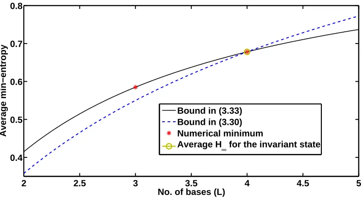
which also gives a lower bound on the Shannon entropy. We prove a lower bound for min-entropic uncertainty relations for any set of MUBs, and show that symmetry plays a central role in obtaining tight bounds. In fact, we obtain for the first time a tight bound for four MUBs in dimensiond= 4, which is attained by an eigenstate of the permuting unitary transformation.

As mentioned earlier, the security of protocols in recent cryptographic models like the bounded-storage and noisy-bounded-storage models is directly related to entropic uncertainty relations. EURs also figure prominently in the security analysis of quantum key distribution [72, 106] and information locking protocols [38]. A better understanding of the interplay between complementarity and uncertainty relations is thus of interest not only from a foundational standpoint, but has practical implications for analyzing and improving existing cryptographic protocols.

1.4

Thesis Organization

(18)

Chapter 2

Approximate Quantum Error

Correction Using the Transpose

Channel

Quantum error correction (QEC) is one of the cornerstones of quantum information and quantum computing. Since quantum effects are extremely fragile and susceptible to damage by environmental noise, QEC plays an important role in making the theoretical idea of quantum information process-ing a physically realizable prospect. Many tasks in quantum communication or computation would indeed become impossible without the use of error-correcting techniques to protect the information from noise. The idea behind QEC is a very simple one—information is stored in a particular part of the system Hilbert space, cleverly chosen depending on the noise process affecting the system, such that a recovery operation can be applied to retrieve the information.

A vast majority of existing work on error correction focuses on the standard paradigm ofperfect

(19)

protection from the noise. While examples of good approximate QEC (AQEC) codes are known, characterizing these approximately correctable codes has remained an open problem.

In this chapter,1 we formulate a simple approach to characterizing and finding AQEC codes. We demonstrate for the first time that there exists a universal, near-optimal recovery map for AQEC codes—the transpose channel—where optimality is defined in terms of the worst-case fidelity. Using the transpose channel, which is constructed as a generalization of the recovery channel defined in [8], we obtain a set of conditions for AQEC, which forms the basis of a simple algorithm for finding AQEC codes. Our analytical approach is a departure from earlier work which relies on exhaustive numerical search for the optimal recovery map, with optimality defined in terms of averageor entanglement fidelity rather than the worst-case fidelity. Furthermore, for the practically useful case of codes encoding a single qubit of information, our algorithm is particularly easy to implement.

The rest of the chapter is organized as follows. In Section 2.1 we briefly review the standard paradigm of quantum error correction. In Section 2.2 we introduce the notion of approximate error correction with an example, and formulate the problem of finding AQEC codes as an optimization problem. In Section 2.3, we define the transpose channel, examine its role in standard QEC theory, and prove that it is nearly optimal for AQEC codes. An alternative form of the perfect QEC conditions based on the transpose channel is described in Section 2.4, a perturbation of which leads to a set of AQEC conditions. The algorithm for finding AQEC codes is described in Section 2.5. In Section 2.6, we consider the example of amplitude damping noise and use it to compare our procedure with earlier work on approximate codes. Section 2.7 contains our conclusions and some open problems.

2.1

Quantum Error Correction

The basic idea of quantum error correction is to encode the information that we wish to protect into a larger quantum system. Specifically, information is stored in quantum states, which are represented bydensity operators ρ _{∈ B}(_H), in a finite-dimensional Hilbert space _H. The operator

ρ is a positive semi-definite, trace-1, linear operator in H. If the state of the system is exactly

1_{The work described in this chapter has been done in collaboration with Hui Khoon Ng. The original results}

(20)

known, it is described by a pure state_|ψ_{i ∈ H}, where_|ψ_i is a unit vector in_H. Density operators corresponding to such pure states are given by ρ = |ψihψ|. Finally, if a system is known to be in state _|ψii with probability pi, where {|ψii, i = 1, . . . , N} is a set of N pure states, it is said

to be in a mixed state and the density operator describing the state of the system is given by

ρ=P_ipi|ψiihψi|.

Figure 2.1: Schematic representation of quantum error correction.

Given the system Hilbert space_H, we seek to encode a qudit of information—information carried by a d-dimensional Hilbert space _H0—where d is no greater than the dimension of H. Often the

system Hilbert space_His simply ann-fold tensor product of the system we seek to encode, that is, H= (_H0)⊗n. The qudit is encoded into ad-dimensional subspaceCofH. Whend= 2, this reduces

to the problem of encoding a single qubit of information, which is of utmost practical relevance today. We refer to_Cas asubspace code, as opposed to subsystem codes [82] or more general codes in the sense of [19]. Since we are only concerned with subspace codes in this chapter, we will often use “code” to denote the subspace_C. Formally, the information is encoded into_C via an encoding map W :H0 → C, whose action on any orthonormal basis{|φ(0)i i} forH0 is W :|φ(0)i i 7→ |φii ∈ C such

that_hφi|φji=δij ∀i, j. One can extend this encoding map on the vector spaceH0 to a completely

positive (CP), trace-preserving (TP) map on operators, also denoted by W.

(21)

noise acting on the system over some timestep, or the effect of a single use of a noisy channel for communication. After the action of E, we perform a CPTP recovery map R : B(H) → B(C) to undo the effects of the noise, and then decode using _W−1. Note that, when a single qudit (qubit) is encoded into n qudits (qubits), the corresponding noise channel is also ann-fold tensor product space of a single qudit (qubit) noise channel_E, denoted as_E⊗n_{. The key steps in the error}

correction process described here are summarized schematically in Fig. 2.1. We will now proceed to describe the quantum noise model in greater detail with examples of some physically motivated noise processes.

2.1.1 Quantum Channels

Formally, any quantum operation on a system can be described by a completely positive, trace preserving (CPTP) map on density operators in the system Hilbert space. A map _E acting on density operators ρ∈ B(HA) is said to completely positive if and only if, (a) E(ρ) >0, ∀ ρ >0∈

B(_HA), and (b) E ⊗IB is a positive map onB(HA⊗ HB), for any possible extensionHA⊗ HB of

the system Hilbert space HA, where IB is the identity map on HB. Condition (a) is the simple

statement that if ρ _{∈ H}A is a valid density operator, then so is E(ρ) (up to normalization). The

additional requirement of complete positivity in condition (b) is the physical requirement that (_{E ⊗}I_B₎₍_ρ_AB_{) also be a valid density operator for any joint state}_ρ_AB _{∈ B}₍_H_A_{⊗ H}_B_{), where}_E _acts

only on the subsystem HA.

Since tr[_E(ρ)] is the probability that the process represented by _E occurred, given the initial state ρ, conservation of probability requires that tr[E(ρ)] = 1 for all ρ. WhenE describes processes where some extra information is obtained by a measurement, then_E could be non-trace-preserving, that is, tr[E(ρ)]≤1. But since we deal with deterministic noise processes here, the corresponding maps are indeed trace-preserving.

It turns out that these physically motivated requirements lead to an elegant mathematical description of quantum operations. The celebrated result due to Choi and Kraus [25, 79, 80] states that a map E :B(H) → B(H) is completely positive if and only if there exists a set of operators {Ei}Ni=1—referred to as aKraus representation ofE—such that the action ofE onρ ∈ B(H) is

given byE(ρ) =PN_i₌₁EiρE_i†. Henceforth, we will denote E with a particular Kraus representation

(22)

to the map _E. Further, the Kraus representation of a CP map is not unique—any two Kraus representations{Ei}Ni and {Fk}Ni such thatFk=PikuikEi, for someN×N unitary matrix (uij),

describe the same map [98, Theorem 8.2]. Finally, the fact that _E is trace-preserving implies that the Kraus operators of E satisfy

X

i

E_i†Ei =I,

whereI _{is the identity operator for the domain of}_E_.

To summarize, quantum noise processes or quantum channels are modeled as CPTP maps on the system Hilbert space, with the individual errors given by the Kraus operators in the operator-sum representation described above. We conclude this section with some concrete examples of single qubit quantum channels.

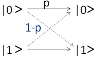
(i) Bit flip channel: The simplest quantum channel we can construct is one that simply flips the state of a qubit from_|0_ito _|1_iwith probability 1₋p. This is a straightforward generalization of the corresponding classical channel which flips the value of a bit with probability 1−p, to the quantum setting. In the_{|0_i,_|1_i} basis, the Kraus operators of this channel are given by

Figure 2.2: The quantum bit flip channel.

E0 =√pI=√p



 1 0

0 1 

; E₁ =p1−p X =p1−p 

 0 1

1 0 

.

(23)

on any state ρcan be described in terms of the Pauli operators as The Kraus operators corresponding to this channel are therefore given by

EDep(ρ)∼ {

p

1−3p/4I_,√_pX/₂_,√_{pY /}₂_,√_pZ/₂_}_.

(iii) Amplitude damping channel: This is an important quantum channel that describes energy dissipation and characterizes the effects due to loss of energy from a quantum system. The single qubit amplitude damping channel EAD has Kraus operators

E₀AD=

written in some qubit basis{|0i,|1i}. EAD can be thought of as describing energy dissipation

in a two-level system, where _|0_i is the ground state and_|1_i is some excited state. γ is then the probability of a transition from the excited state to the ground state. In the Pauli basis,

E₀AD= 1

showing that no linear combination ofE0 and E1 can give an operation element proportional

to the identity operator. The fact that the operator elements of the amplitude damping channel cannot be realized as scaled Pauli operators makes it different from the other two channels described here.

2.1.2 Perfect QEC Conditions

(24)

R leaves states in the codespace _C unaffected. Formally, the action of a channel _E is said to be

perfectly correctible on a codespace C _{if and only if there exists a quantum channel} _R _{such that}

R ◦ E(ρ) = ρ _∀ρ _∈ C_.

An important characterization of perfect QEC codes is given by the perfect QEC conditions [15, 43, 70], which we briefly review here. For a given code_C, letP be the projector onto _C. The QEC conditions can then be stated as follows.

Theorem 2.1.1 (Perfect QEC conditions[15, 43, 70]). A CPTP recovery mapR that perfectly corrects the action of a noise channel_{E ∼ {}Ei}Ni=1 on a subspace code C exists, if and only if

∀i, j, P E_i†EjP =αijP, (2.3)

for some complex matrix α.

Note that this is simply a condition on the existence of a perfect QEC code for a given E, and stipulates no knowledge of the recovery map_R.

It is more insightful to rewrite (2.3) in a “diagonal” form. From (2.3), it is clear thatαmust be a Hermitian matrix. Therefore, there exists a unitaryuand a diagonal matrixdsuch thatα =udu†. The set of operators defined byFk≡PiuikEi constitutes an alternate Kraus representation forE,

so that _{E ∼ {}Fk}. With this choice of Kraus representation, the perfect QEC condition takes the

following form:

∀k, l, P F_k†FlP =δkldkkP, (2.4)

wheredkkare the diagonal entries ofd, or equivalently, the eigenvalues ofα. Notice thatdkk≥0, ∀k,

since the left-hand side of (2.4) is positive semi-definite when k = l. α is hence a positive semi-definite matrix (α_≥0).

The diagonal form of the perfect QEC condition makes it easier to appreciate the intuition behind Theorem 2.1.1. Using polar decomposition, we can express the Fk’s as FkP =√dkkUkP,

for unitaryUk. The effect of the Kraus operators on a perfect code is therefore unitary, in the sense

that the operator Fk simply rotates the codespace C into the subspace defined by the projector

Pk ≡UkP Uk†. Equation (2.4) further guarantees that these projectors are orthogonal, that is,

PkPl=UkP Uk†UlP Ul†=

UkP F_k†FlP U_l†

(25)

thus implying that the individual errors due to the action of the channel can be reliably distinguished by a projective measurement. The individual error operators of a noise channel thus map a perfectly correctible codespace to mutually orthogonal subspaces of the encoding Hilbert space, as shown in Fig. 2.3.

Figure 2.3: Action of noise on perfectly correctible code.

The recovery map for correcting the errors when (2.3) is satisfied, is now easy to construct. Let us denote this recovery as Rperf. To write down Rperf, we use the polar decomposition to obtain

the unitaries Uk such thatFkP =√dkkUkP. Then, Rperf :B(PE)→ B(C) is given by

Rperf∼ {P Uk†}.

One can check thatRperfis TP on its domainB(PE), and that it perfectly corrects the code in the

sense that for anyρ_{∈ B}(_C),

(Rperf◦ E)(ρ) =

X

k

dkk

ρ. (2.5)

P

kdkk is just the trace ofE(ρ) for any ρ ∈ C. This sum is independent ofρ because of the QEC

conditions (2.4), and is exactly equal to 1 if and only if_E is TP on _C. Equation (2.5) thus implies thatRperfrecovers the original code state, up to any reduction in trace due to the possible non-TP

nature of _E.

(26)

checkable for a given codespace _C. Furthermore, (2.3) is linear. If _{E ∼ {}Ei} is correctible on

codespace C, then any channel whose operator elements are linear combinations of {Ei} is also

correctible. Since the Pauli matrices form a basis for 2_×2 matrices, this linearity property has the important consequence that for correcting single qubit errors, it suffices to check that a given code satisfies the condition for the “Pauli errors,” namely the operators (I_{, X, Y, Z}_).

It turns out that the smallest code capable of perfectly correcting an arbitrary error on any single qubit of the system, requires five qubits. This can be shown to follow from the linearity of the error-correcting condition (2.3) and the assumption that errors act independently on different qubits. We refer to [98, Section 10.3.4] for detailed proofs that any general quantum code that seeks to correct single qubit errors perfectly, must encode into atleast 5 qubits. The five-qubit code [15, 84] is thus the shortest known perfect QEC code. We will henceforth refer to this as the as the [[5,1,3]] code, where the first entry in the brackets corresponds to the number of qubits in the system, and the second entry is the number of qubits of information encoded in the system. The third entry is the distance of the code, defined asd= 2t+ 1 where tis the maximum number of qubits that the code can perfectly correct. Since the five-qubit code is capable of correcting any error on a qubit, its distance parameter is equal to 3. This code satisfies the perfect QEC conditions for any noise channelE⊗5_{, but with terms corresponding to more than a single-qubit (Pauli) error}

discarded.

2.2

Approximate Quantum Error Correction

(27)

behind the success of their code. Such approximate QEC (AQEC) codes reveal the possibility of designing codes that are better tailored to the particular information processing task at hand. Before proceeding to analyze the problem of characterizing such approximately correcting codes, it will help to gain some intuition into the working of this four-qubit code.

2.2.1 The Approximate [4,1] Code

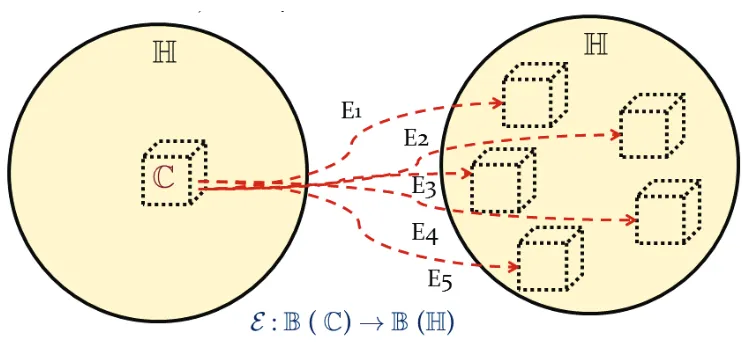
The four-qubit code constructed by Leung et al. [85] protects a single qubit of information against amplitude damping noise by encoding into four physical qubits. Assuming that the noise acts independently on the qubits, the four-qubit noise channel is just four copies of _EAD, that is, EAD⊗4.

The four-qubit subspace code constructed in [85] is the span of the following two states:

|0Li ≡

want to encode in the four-qubit Hilbert space. We denote this as the [4,1] code, where as before, the first entry in the brackets corresponds to the number of qubits in the system, and the second entry is the number of qubits of information encoded in the system. It was shown in [85] that this code satisfies the perfect QEC conditions for EAD⊗4, except for small corrections of order γ2. If

PL = |0Lih0L|+|1Lih1L| denotes the projector onto the codespace, the Kraus operators {EiAD}

corresponding to the four-qubit channelEAD⊗4 satisfy

PL(EiAD)†EjADPL= 0, i6=j;PL(EiAD)†EiADPL=PLDiPL, (2.7)

Comparing (2.7) with the perfect QEC condition (2.3), we see that here, while the Kraus operators map the codespace (defined in (2.6)) to mutually orthogonal subspaces, these subspaces are not

unitary transformations of the codespace. This is schematically represented in Fig. 2.4.

As in the case of perfect QEC, a recovery operation similar to _Rperf can be constructed to

approximately correct for single qubit errors in the [4,1] code. Polar decomposition of the Kraus operators EAD

k PL = UkL

√

(28)

Figure 2.4: Action ofEAD⊗4 on the [4,1] code.

given byRL≡ {PL(U_kL)†}. We compare the performance of the [4,1] code with that of the perfect

[[5,1,3]] code and other approximate codes in Section 2.6.

2.2.2 AQEC as an Optimization Problem

While the analysis in [85] is based on investigating small perturbations of the perfect QEC condi-tions, recent work has focused on solving AQEC as an optimization problem. Indeed the challenge of AQEC is to find the optimal encoding and recovery maps, given a noise channel and the infor-mation we want to encode (qubit or higher-dimensional object), with optimality defined in terms of a chosen measure of faithfulness between the input state and the recovered state.

The fidelity between the input qudit state and the decoded state after noise and recovery quantifies how well the information is protected from the noise. The fidelity between any two states ρand σ is given by

F(ρ, σ)≡tr q

ρ1/2_σρ1/2_,

which for a pure state ρ≡ |ψihψ|, can be written as

(29)

For anyρandσ,F(ρ, σ) takes value between 0 and 1. F = 0 if and only ifρandσ have orthogonal support, andF = 1 if and only if ρ=σ. The fidelity hence gives a measure of how close two states are.

We say that a code C, together with its encoding and recovery maps, is effective at protecting the information from the noise _E if theworst-case fidelity

min

ρ∈S(H0)F

ρ, _W−1_{◦ R ◦ E ◦ W} ρ (2.8)

is close to 1. Here, _S(_H0) denotes the set of all states, pure or mixed, of the qudit. In practice, it

suffices to minimize over pure states in S(H0) only, since the fidelity measure is jointly concave in

its arguments. Concavity implies that for any probability distribution pi and density operators ρi

and σi,

Since this is true for all states ρ∈ S(H0), the minimum fidelity is clearly attained on a pure state.

Setting Φ_{≡ W}−1_{◦ R ◦ E ◦ W}_{, we see that the minimization in (2.8) needs to be performed only}

over pure states.

Equation (2.8) defines the worst-case fidelity for a given encoding map (or equivalently a given code C ⊂ H) and a given recovery map. In reality, one wants to maximize the error correction capability by choosing_W and _R such that the worst-case fidelity is as close to 1 as possible. The problem of AQEC can thus be phrased as the following triple optimization problem:

max

W maxR |ψmini∈H0

(30)

If the quantity in (2.10) attains the maximum possible value of 1, that is, if there exist _W and _R such that the worst-case fidelity is 1, then we have perfect QEC. In reality, one should also allow H to vary, and choose the smallest possible _H that can accommodate a code with good fidelity performance. For example, in the case of a system consisting ofnquantum registers, one would like to minimize n to reduce resource requirements. Choosing a Hilbert space that is too small might however reduce the worst-case fidelity of possible codes, so one would need to seek an optimal balance between having a smalln and having high fidelity.

A simple approach to estimate (2.10) is to fix either the encoding or the recovery map, and then perform the optimization over the remaining two variables—the recovery or the encoding map, and the input state. Past work on finding optimal AQEC codes [46,48,77,78,105] has for the most part focused on the simpler problem of optimizing for measures based on entanglement fidelity [117], which characterize the performance of the code averaged over some input ensemble (including the case of a trivial ensemble comprising a single state). This eliminates the minimization over all input states required for the worst-case fidelity measure. The task of finding the optimal encoding or recovery map is then tractable via convex-optimization methods, but the resulting recovery is now optimal for an averaged measure of fidelity. Recovery maps which are near-optimal for the average entanglement fidelity have been constructed analytically [8, 124]. Conditions for AQEC based on the worst-case entanglement fidelity have also been formulated recently [17].

For many communication or computational tasks, however, one would prefer an assurance that

all the information stored in the code is wellprotected. In such cases, theworst-case fidelitydefined above (2.8) is the appropriate measure for determining the optimality of encoding and recovery maps. The resulting double-optimization problem for a given encoding map was examined using semi-definite programming in [135]. This method however requires a relaxation of one of the constraints in the problem, so the recovery map found is typically suboptimal. Furthermore, the numerically computed recovery map is difficult to describe and understand analytically.

(31)

given _W and _R, the worst-case fidelity can as well be computed over states in _C instead of _H0.

Therefore, the relevant optimization problem is

max

R |minψi∈CF[|ψi,(R ◦ E) (|ψihψ|)]. (2.11) Estimating (2.11) for a given code spaceCis a difficult problem since it involves a double optimiza-tion. In our work, we approach the problem stated in (2.11) using a universal recovery map that is analytically very simple to write down, and provably near-optimal, with optimality defined with respect to the worst-case fidelity.

Before proceeding further, let us define some useful terminology. We will often make use of the square of the fidelity, which we denote as F2₍_·_,_·₎_≡_[_F₍_·_,_·_)]2_{. Whenever it is unambiguous, we will}

also refer toF2 as the fidelity. It is also convenient to define the fidelity loss ηR, for a given code C and a recovery map_R, as the deviation of the square of the worst-case fidelity from 1, that is,

ηR≡1− min |ψi∈CF

2_[_|_ψ_i_,₍_{R ◦ E}₎₍_|_ψ_ih_ψ_|_)]_. _(2.12)

The fidelity loss for the optimal recovery mapRop is denoted byηop, and is given byηop= minRηR for a given _C (which is just a restatement of (2.11)). We refer to ηop as the optimal fidelity loss.

A code C for E is said to be -correctable if it has ηop ≤ for some ∈ [0,1]. -correctable

codes with 1 are said to be approximately correctable, and have states with fidelity at least √

1−'1−/2 after the action of the noise and recovery.

2.3

The Transpose Channel

Using the worst-case fidelity measure to define optimality, and assuming a fixed encoding, we now demonstrate a universal recovery map—the transpose channel—which gives a worst-case fidelity that can be suboptimal, but cannot be too far from that of the optimal recovery. First, we establish that this transpose channel is exactly the standard recovery map for perfect QEC codes character-ized by the QEC condition (2.3). Then, we show that the transpose channel is nearly optimal even in the case of AQEC codes.

We begin this section with a description of the transpose channel. For a given code _C, let P

(32)

Let _{Ei}Ni=1 be a Kraus representation for E. The transpose channel RP : B(PE) → B(C) for the

given C is defined as the following CPTP map:

RP(·)≡ N X

i=1

P E_i†_E(P)−1/2(_·)_E(P)−1/2EiP,

i.e., _RP ∼ {P Ei†E(P)−1/2}Ni=1. The inverse of E(P) is taken on its support PE. RP has this

universal form for any channel _E and any code _C, and depends on _C only through P. _RP is a

special case of a recovery map introduced in [8] for reversing the effects of a quantum channel on a given initial state. In fact the _RP is exactly the recovery map for the initial state P/d, where

dis the dimension of C. In [19], RP was shown to be useful for correcting information carried by

codes preserved according to an operationally motivated notion. The term transpose channel owes its origin to [99], where this channel was first defined in an information-theoretic context. It was shown [101] that the transpose channel has the property of being the unique noise channel that saturates Uhlmanns theorem on the monotonicity of relative entropy – a fact that was later used to characterize states that saturate the strong subadditivity of quantum entropy [55].

Observe that the Kraus operators of RP satisfy

X

i

(P E_i†_E(P)−1/2)†(P E_i†_E(P)−1/2) =PE,

soRP is TP on its domain, B(PE). Note that we can always add an additional projector (I−PE) – corresponding to doing nothing on the complement of _PE—to the Kraus operators of _RP, thus

rendering it TP on the full H and making it a valid physical operation on the system. However, since we assume that the information is encoded completely within the code space, the action of RP outsidePE is irrelevant, so we can ignore this extension outside PE.

We can understand the transpose channel as being composed of three CP maps: _RP =

P ◦ E†◦ N, where _P is the projection P(_·)P onto _C, and _N is the normalization map _N(_·) = E(P)−1/2(_·)_E(P)−1/2. In this form, _RP is manifestly independent of the choice of Kraus

repre-sentation for _E. Without the map _N, _RP is just the adjoint map E† ∼ {E_i†} with an additional

projection to ensure that we end up inB(C). However, P ◦ E†_{is not TP, and} _N _{is added precisely} to remedy that.

(33)

perfect QEC codes provides the intuition behind the AQEC conditions presented later.

2.3.1 The Transpose Channel for Perfect QEC

A natural question to ask here is how the transpose channel _RP relates to the recovery Rperf for

a given E and C that satisfy the QEC conditions. Here, we show that they are exactly the same map, as previously noted in [8].

which are exactly the Kraus operators of_Rperf. Thus, we see that when the perfect QEC conditions

are satisfied, RP is exactly the optimal recovery map that perfectly correctsE on C.

Note that Theorem 2.1.1 and Lemma 2.3.1 remain true even for an _E that is not TP. Tradition-ally, perfect QEC is discussed for a noise channelE that is CP but not necessarily TP. The non-TP case is particularly relevant when we deal with a system ofnquantum registers, with each register independently affected by some noise E1. Then, instead of requiring the code to correct the entire

noise channel_E₁⊗n, one often looks for codes that perfectly correct the noise up to some maximum number tof quantum registers with errors. In this case, we takeE as the channel describing noise where at mostt registers have errors, instead of the full noise channel _E₁⊗n. Such an _E is not TP, since we have discarded the part ofE1⊗n that corresponds to having errors in more thantregisters.

(34)

Actually, a perfectly correctable code for such a non-TP noise channel can be viewed as an approximately correctable code for the original n-register noise channel E1⊗n, which is TP. In our

AQEC discussion, the code we look for is approximately correctable on the channel anyway, so _E is always assumed to be TP, which is the physically relevant scenario. Note that the analysis in the remainder of the paper does apply for a special type of non-TP maps—_{E ∼ {}Ei} satisfying P

iP E

†

iEiP =aP, wherePis the projector onto the code space and 0≤a≤1. Our analysis applies

in this case, except that one would have to add the proportionality factor ato our expressions.

2.3.2 Near-Optimality of the Transpose Channel

For AQEC codes, while the transpose channel _RP need not be the optimal recovery mapRop, we

show that_RP does nearly as well asRop. This is our central result and forms the basis of much of

the discussion that follows.

Theorem 2.3.2. Given a subspace code _C of dimension d and optimal fidelity loss ηop, for any

|ψi ∈ C,

where _h._i denotes the expectation value with respect to the state _|ψ_i. Since _Rop is TP, we have

(35)

construction, we get

hψ|(Rop◦ E)(P)|ψi=hψ1| d X

i=1

ρi|ψ1i

=α(1)₁₁ +

d X

i=2

α(₁₁i)_≤1 + (d₋1)ηop.

Putting this back into (2.15), and noting that hP_i_|hE_i†_E(P)−1/2Eii|2 i1/2

≤F(_|ψ_i,_RP ◦ E) gives

F2[_|ψ_i,(_Rop◦ E)(|ψihψ|]≤

q

1 + (d₋1)ηopF[|ψi,(RP ◦ E)(|ψihψ|)], (2.16)

which proves the theorem.

Let ηP denote the fidelity loss for code C with the transpose channel RP as the recovery map.

Then, Theorem 2.3.2 implies the following corollary.

Corollary 2.3.3. ηP satisfies ηop≤ηP ≤ηopf(ηop;d), where f(η;d) is the function

f(η;d)_≡ (d+ 1)−η

1 + (d−1)η = (d+ 1) +O(η). (2.17)

Proof. That ηP ≥ηop is true by the definition of ηop. To show that ηP ≤ηopf(ηop;d), define for

any _|ψ_{i ∈ C},ηP,ψ such that F2[|ψi,(RP ◦ E)(|ψihψ|)]≡1−ηP,ψ. ηP is then justηP ≡maxψηP,ψ.

From Theorem 2.3.2, we see that

1−ηop ≤F2[|ψi,(Rop◦ E) (|ψihψ|)]

≤q1 + (d−1)ηop F[|ψi,(RP ◦ E)(|ψihψ|)]

=q[1 + (d₋1)ηop] (1−ηP,ψ).

Rearranging gives ηP,ψ ≤ηopf(ηop;d). Since this holds for allηP,ψ, it also holds forηP.

The inequality ηP ≤ ηopf(ηop;d) makes precise our statement that RP is near-optimal. The

recovery RP works nearly as well as the optimal recovery, since its fidelity loss picks up at most

(36)

that when ηop = 0, the inequality in Corollary 2.3.3 reduces to ηP =ηop, reaffirming that RP is

the optimal recovery in the case of perfect QEC.

We do not know if the upper bound onηP in Corollary 2.3.3 is tight. However, the appearance

of the dimension d of the code in the bound is unavoidable, as can be seen from the following example. Consider a noise channel_{E ∼ {}Ei}such that the action ofEon a codeCcan be described

by the set of Kraus operators {EiP} = {√1−p P,√p |0ih0|,√p |0ih1|, . . . ,√p |0ihd−1|}, for

0 _≤ p 1. As usual, P is the projector onto _C and d is the dimension of _C. _E mostly acts like the identity channel on C, but has a small component that maps a small part of every code state onto the state _|0_i. For d_≥3, one can show that the worst-case fidelity, when using the transpose channel as the recovery, occurs for the state |0i. The corresponding fidelity loss is

ηP =

(d−1)p

1 + (d−1)p. (2.18)

On the other hand, sinceE is nearly the identity channel, we can perhaps not do any recovery, i.e., make the identity channel the recovery map. In this case, we find that the fidelity loss is η0 ≡ p

which is always smaller than ηP for small p. Since the optimal fidelity loss ηop must always be

smaller thanη0, we have thatηP/ηop ≥ηP/η0 = (d−1)/[1+(d−1)p], which grows asdincreases, for

fixedp. Therefore, we see that there is an increasing separation between ηP andηop asdincreases.

In the next section, we will see that this approach to AQEC using the transpose channel can be viewed as a perturbation from the perfect QEC case. The factor ofdappearing in our bounds can perhaps be understood as quantifying the number of degrees of freedom in which the approximate case can deviate from the perfect case. Note, however, that asdgets large, f(η;d) approaches 1/η. In this case, the inequality in Corollary 2.3.3 simply becomes the trivial statement ηop ≤ηP ≤1.

While we will often only be interested in codes with small values of d, this demonstrates the weakness in the bounds derived here for large values of d.

Finally, note that Corollary 2.3.3 provides a necessary and sufficient condition for C to be ap-proximately correctable—_C is approximately correctable if and only if ηP is small. In the next

(37)

2.4

The Transpose channel and QEC Conditions

One of the key tools in perfect QEC are the QEC conditions stated in Theorem 2.1.1. Similar conditions characterizing AQEC codes would be very useful. A natural approach to getting a set of AQEC conditions is to perturb the perfect QEC conditions to allow for small deviations. For example, the four-qubit code for the amplitude damping channel described in Section 2.2.1 was shown to obey a set of perturbed QEC conditions. More recent studies [90] have looked at small perturbations of the perfect QEC conditions for general CPTP channels. However, the analysis in [90] is complicated, and one wonders if there is a simpler approach using the transpose channel. In this section, we prove a simple set of AQEC conditions based on Corollary 2.3.3. Drawing from our earlier observation that the transpose channel is the optimal recovery map for perfect QEC codes in Lemma 2.3.1, we rewrite the condition (2.3) for perfect QEC in such a way that the role of the transpose channel is apparent. From this, we derive a necessary and a sufficient condition for AQEC founded upon the transpose channel, as a natural generalization of the perfect QEC conditions. While AQEC conditions have been derived in the past from information-theoretic perspectives [16, 20, 69, 118], our conditions are algebraic, and lead to a simple and universal algo-rithm to find AQEC codes that does not require optimizing over all recovery maps for each encoding map.

2.4.1 Alternative Form of the Perfect QEC Conditions

The role of the transpose channel in perfect QEC becomes a lot more transparent once we realize that the QEC conditions in Theorem 2.1.1 can be written as follows.

Theorem 2.4.1 (Alternative perfect QEC conditions). A code _C satisfies the perfect QEC conditions of Theorem 2.1.1 if and only if it satisfies

∀i, j, P E_i†E(P)−1/2EjP =βijP, (2.19)

where β ≡√α, for α from Theorem 2.1.1.

Proof. For a code C that satisfies the perfect QEC conditions, using (2.13) and P U_k†UlP = δklP,

we have

P F_k†E(P)−1/2FlP = p

dllP Uk†UlP =δkl p

(38)

This diagonal form can be rotated to any other Kraus representation by using the appropriate unitary u, such that Fk = PiuikEi and α = udu†. Then, defining β ≡ √α, we get (2.19), thus

showing that a code_C satisfying the perfect QEC conditions, also satisfies (2.19).

Conversely, suppose we start with the “diagonal” form of (2.19) as in (2.20), which can be accomplished by choosing a unitary u so that β is diagonal with entries √dkk. Since E is CP,

E(P) ≥ 0 and hence E(P)−1/2 ≥ 0. Therefore, we can take square root of (2.20) and write

which is exactly the diagonal form of the perfect QEC conditions (2.4). Applying an appropriate

u to rotate to the desired Kraus representation gives (2.3).

It may be observed that the left-hand side of (2.19) is simply a Kraus operator of the map_RP◦E.

In other words, the QEC conditions given in Theorem 2.4.1, as also the original version given in Theorem 2.1.1, simply express the fact that C is perfectly correctable if and only if RP ◦ E ∝ Pˆ,

where ˆ_P is the projection P(_·)P, which acts trivially on the code_C. The proportionality factor is P

ijβij2 = P

ijαij =Pkdkk.

2.4.2 AQEC Conditions

We now obtain conditions for AQEC by perturbing the alternative form (2.19) of the perfect QEC conditions. The perturbation is added as a small operator on the right-hand side of (2.19) for each

(39)

Corollary 2.3.3.

Theorem 2.4.2 (AQEC conditions). Suppose we have a CPTP channel _{E ∼ {}Ei}, and a d -dimensional subspace code C with projector P. Let ∆ij ∈ B(C) be traceless operators such that

P E_i†E(P)−1/2EjP =βijP+ ∆ij, (2.22) where βij ∈C. Then, for ∈[0,1], there existsη ∈[0,1] such that

(i) C is -correctable if η≤;

(ii) _C is -correctable only if η_≤f(;d), where f is the function

f(;d)≡ (d+ 1)−

1 + (d−1) = (d+ 1) +O(). (2.23)

Proof. The left-hand side of (2.22) are Kraus operators of _RP ◦ E. This, along with the fact that

RP ◦ E is trace-preserving, implies that for a noise channel E satisfying (2.22), the fidelity under

the transpose channel recovery is given by

F2[|ψi,(RP ◦ E)(|ψihψ|)] = 1− X

ij h

hψ|∆†_ij∆ij|ψi − |hψ|∆ij|ψi|2 i

. (2.24)

Recalling the definition of the fidelity loss ηP, for the transpose channel, we get

ηP = max

|ψi∈C X

ij h

hψ|∆†_ij∆ij|ψi − |hψ|∆ij|ψi|2 i

. (2.25)

Settingη =ηP, conditions (i) and (ii) follow directly from Corollary 2.3.3.

It is clear that the expression for ηP is a non-negative quantity, since the fidelity in (2.24) is

bounded by 1. Furthermore, (2.25) elucidates how the fidelity loss arises from the presence of the ∆ij operators. If ∆ij = 0 ∀i, j, we have perfect QEC.

(40)

E are known. If ηP ≤, thenC is a good code. If however,ηP violates the inequality in Condition

(ii), we know thatC is not good enough for our purposes. Of course, there is a gap—for ηP taking

values _≤ ηP ≤ f(;d), we cannot use these conditions to determine whether C is within our

tolerable fidelity loss, but this gap is small for smalld. We do not know if the gap can be shrunk by replacing ηP with the fidelity loss for a recovery map other than the transpose channel, but we

believe it is unlikely to vanish completely.

For a general _C, the fidelity lossηP may be difficult to compute as it requires a maximization

over all states in the code space. However, there is a quick way to check for sufficiency by relaxing condition (i) of Theorem 2.4.2 slightly.

Corollary 2.4.3. _C is-correctable for some _∈[0,1] if

k∆sum k ≤, (2.26)

where ∆sum≡Pij∆

†

ij∆ij and k · k denotes the operator norm. Proof. Observe that P_ij[_hψ_|∆†_ij∆ij|ψi − |hψ|∆†ij|ψi|2] ≤

P ijhψ|∆

†

ij∆ij|ψi = hψ|∆sum|ψi. From

the definition of the operator norm, it is easy to see that max|ψi∈Chψ|∆sum|ψi = k∆sumk. Hence,

ηP ≤ k∆sumk, and the conditionηP ≤in statement (i) of the AQEC conditions (Corollary 2.3.2)

is certainly satisfied ifk∆sumk ≤.

This sufficiency condition (2.26) and the AQEC conditions of Theorem 2.4.2 form the basis of a simple algorithm to find good AQEC codes, presented in the next section. Since ∆sum is

a positive semi-definite operator, its operator norm is given by its maximum eigenvalue, which is easily computable. In fact, for codes encoding a single qubit, we show in Appendix A that k∆sumk= 1−P_ij|βij|2. Note that for a given codeC and noise channel E,βij is easily computed,

since βij = (1/d) tr[P Ei†E(P)−1/2EjP]. Furthermore, we also show in Appendix A that for the

case of qubit codes, ηP can be computed easily with simple eigenanalysis. In fact our method of

(41)

2.5

Finding AQEC Codes

Consider the practical problem of finding a d-dimensional code, given some maximum tolerable fidelity loss, such that, every code state must have fidelityF _≥√1₋, after passing through the noise channel and recovery map. The following algorithm provides a simple procedure to search for such -correctable codes, for a given noise channel and system Hilbert space.

Algorithm

Step 1. Pick ad-dimensional subspace_{C ⊆ H}. This can be done, for example, by randomly picking

dlinearly independent vectors from Hand defining C as their linear span. Step 2. Compute∀i, j,

∆ij ≡P Ei†E(P)−1/2EjP −βijP, (2.27a)

βij ≡

1

d tr(P E

†

iE(P)−1/2EjP). (2.27b)

Find the maximum eigenvalue λmaxof ∆sum≡Pij∆

†

ij∆ij. Ifλmax≤, then we are done,

since_C is an-correctable code.

Step 3. If not, compute the fidelity lossηP for the recovery map RP, as given in (2.25). IfηP ≤,

then again C is an-correctable code.

Step 4. If not, check if ηP > f(;d). If true,C is not -correctable. We return to Step 1 and try

again with a different_C.

Step 5. If < ηP ≤f(;d), we do not know if Cis-correctable, but we can still choose to discard

this _C and return to Step 1 to try again with a different _C.

(42)

There is of course the possibility that the algorithm yields no code within our fidelity loss requirements. This does not immediately imply that H does not contain an -correctable code, because of the presence of the gap stated in Step 5. However, figuring out whether any of the codes that fall in this gap is a good enough code is the same as finding the optimal recovery map for that code, a problem which we currently do not know how to solve efficiently.

2.6

Example: Amplitude Damping Channel

In this section we compare the performance of the transpose channel with that of other AQEC schemes, for the case of amplitude damping noise. The single-qubit amplitude damping channel EAD is the CPTP channel described in (2.2), parameterized by the damping parameter γ. Recall

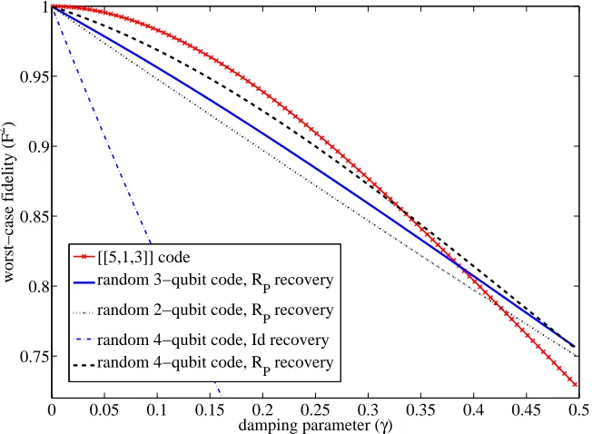
thatγ corresponds to the probability of a transition from the excited state to the ground state. In Fig. 2.5 we plot the worst-case fidelity for different AQEC codes as function of γ.

Clearly, in the absence of any encoding or recovery, the worst-case fidelity for a single qubit undergoingEAD decreases as 1−γ (see Fig. 2.5, line labeled “no error correction”). The [4,1] code

due to Leung et al described in Section 2.2.1, in combination with the Leung recovery, increases the fidelity significantly as compared to the no error correction case. In the same figure, we have also plotted the worst-case fidelity using the transpose channel_RP as the recovery operation instead of

the Leung recovery, for the same [4,1] code. From the plot, we can see that using the transpose channel as the recovery map gives a higher fidelity than the original Leung recovery.

For comparison, we have also looked at a recovery map for the [4,1] code constructed by Fletcher et al. in [47]. Their recovery, which we refer to as the Fletcher recovery, was originally optimized for an averaged measure of fidelity. We have instead computed the worst-case fidelity for this recovery, 2 and this is plotted in Fig. 2.5. For small values of γ, the Fletcher recovery gives the best performance compared to the other recovery maps, despite being optimized for an averaged measure of fidelity. However, it is only marginally better than the transpose channel recovery.

We have also compared the performance of the [4,1] approximate code under these different recovery maps with that of the smallest known perfect code, namely the [[5,1,3]] code [15, 84].

2_{The recovery map we use here is from Table I of [47]. Their recovery map actually depends on two parameters}

αandβ which can be numerically optimized, for each value ofγ, for the best recovery map. For simplicity, we set

(43)

Using the corresponding_Rperf as the recovery for the [[5,1,3]] code, we have computed the

worst-case fidelity for different values of γ. As the plot in Fig. 2.5 shows, the [[5,1,3]] code performs better than the [4,1] code with Leung recovery, but the [4,1] code uses one fewer qubit to encode the same amount of information. The [4,1] code with the transpose channel as recovery has nearly identical worst-case fidelity as the [[5,1,3]] code, while the one with Fletcher recovery does slightly better than the [[5,1,3]] code for small values ofγ.

These observations clearly demonstrate the benefit of going beyond the codes described by the perfect QEC conditions. Furthermore, while the [[5,1,3]] code is capable of perfectly correcting any single qubit error on a system subjected to any noise channel, the comparison with the [4,1] code with its various recovery maps clearly show the gain that one might achieve by adapting the codes and recovery to the noise channel in question.

Finally, we have also randomly generated codes that encode a single qubit into four physical qubits, for the amplitude damping channel. We computed the worst-case fidelity for each code using the transpose channel as the recovery map. We tried about 500 randomly selected codes, taking less than half an hour on a typical laptop computer. The worst-case fidelity for the best code we found is given in Fig. 2.5 (line marked “random 4-qubit code,_RP recovery”). For small values ofγ,

this random code does not do as well as the other codes discussed so far for the amplitude damping channel, but it still does significantly better than the case without error correction. Furthermore, for

γ &0.35, our randomly generated code actually outperforms all the other codes. For comparison, we have also plotted the worst-case fidelity for this randomly generated code in the absence of the transpose channel recovery, i.e., with the identity channel as the recovery map (line marked “random 4-qubit code, Id recovery”). In all this, one should keep in mind the ease with which the performance of the randomly generated code was achieved, due to the fact that the transpose channel is a near-optimal recovery map forany code.

(44)

0 0.05 0.1 0.15 0.2 0.25 0.3 0.35 0.4 0.45 0.5

Figure 2.5: Codes for the amplitude damping channel, for 0≤γ ≤0.5.

0 0.05 0.1 0.15 0.2 0.25 0.3 0.35 0.4 0.45 0.5

(45)

randomly generated four-qubit code mentioned in the previous paragraph. From the figure, we see that while the worst-case fidelity decreases as the number of physical qubits decreases, the two- and three-qubit codes in fact do not perform too badly compared to the four-qubit code or the [[5,1,3]] code. Such codes may be of relevance whenever the desire to lower resource requirements trumps the need for the best possible worst-case fidelity.