Western University Western University
Scholarship@Western
Scholarship@Western
Electronic Thesis and Dissertation Repository
1-22-2014
Oligonucleotide Design for Whole Genome Tiling Arrays
Oligonucleotide Design for Whole Genome Tiling Arrays
Qin Dong
The University of Western Ontario
Supervisor Lucian Ilie
The University of Western Ontario Graduate Program in Computer Science
A thesis submitted in partial fulfillment of the requirements for the degree in Master of Science © Qin Dong 2014
Follow this and additional works at: https://ir.lib.uwo.ca/etd
Part of the Bioinformatics Commons, and the Other Computer Sciences Commons
Recommended Citation Recommended Citation
Dong, Qin, "Oligonucleotide Design for Whole Genome Tiling Arrays" (2014). Electronic Thesis and Dissertation Repository. 1875.
https://ir.lib.uwo.ca/etd/1875
This Dissertation/Thesis is brought to you for free and open access by Scholarship@Western. It has been accepted for inclusion in Electronic Thesis and Dissertation Repository by an authorized administrator of
Qin Dong
Graduate Program in Computer Science
A thesis submitted in partial fulfillment
of the requirements for the degree of
Masters of Science
The School of Graduate and Postdoctoral Studies
The University of Western Ontario
London, Ontario, Canada
c
Abstract
Oligonucleotides are short, single-stranded fragments of DNA or RNA, designed to
readily bind with a unique part in the target sequence. They have many important
applications including PCR (polymerase chain reaction) amplification, microarrays,
or FISH (fluorescence in situ hybridization) probes.
While traditional microarrays are commonly used for measuring gene expression
levels by probing for sequences of known and predicted genes, high-density, whole
genome tiling arrays probe intensively for sequences that are known to exist in a
contiguous region.
Current programs for designing oligonucleotides for tiling arrays are not able to
produce results that are close to optimal since they allow oligonucleotides that are
too similar with non-targets, thus enabling unwanted cross-hybridization. We present
a new program, BOND-tile, that produces much better tiling arrays, as shown by
extensive comparison with leading programs.
Keywords: DNA, oligonucleotide, tiling arrays, microarrays
Thirdly, I sincerely appreciate my boyfriend, Fang Han, for his encouragements
and understanding. My appreciation also goes to Di Yao. As my best friend, she is
my proud of my life.
Last but not the least, I’d like to thank all my lab-mates, especially Yiwei Li
and Ehsan Haghshenas, the good colleagues and friends who offered me support and
information a lot. Without Yiwei’s help, it would take me much more time to finish
my study.
Contents
Abstract ii
Acknowlegements iii
List of Figures vii
List of Tables x
1 Introduction 1
2 Genome Tiling 3
2.1 Molecular biology primer . . . 3
2.1.1 Organisms and cells . . . 3
2.1.2 DNA, RNA, and proteins . . . 4
2.1.3 Genome, chromosome, and gene . . . 6
2.1.4 Thermodynamics of DNA . . . 6
2.2 Oligonucleotides and applications . . . 8
2.2.1 Oligonucleotides . . . 8
2.2.2 Applications of oligonucleotides . . . 9
2.3 Whole Genome Tiling . . . 10
2.4 Sequence alignments . . . 12
2.5 Text indexing . . . 13
2.6 FM-index . . . 14
2.6.1 Burrows-Wheeler transform . . . 15
2.6.2 The FM-index . . . 16
2.7 Leading programs for genome tiling . . . 17
Tiling resolution . . . 22
Thermodynamic properties of oligonucleotide probes . . . 23
Additional Parameters . . . 24
3 BOND-tile 25 3.1 Problems with previous designs . . . 25
3.2 Spaced seeds . . . 26
3.3 The BOND-tile algorithm . . . 28
3.3.1 The outline of BOND-tile algorithm . . . 29
Oligo placement . . . 29
Outline of BOND-tile . . . 30
3.3.2 DNA encoding . . . 30
3.3.3 GC content . . . 31
3.3.4 Melting temperature . . . 32
3.3.5 Similarity search . . . 33
Hash table construction . . . 34
Phase I: Fast elimination . . . 34
Phase II: Intensive search and elimination . . . 35
Differrence between fast and intensive elimination . . . 35
3.3.6 Oligonucleotide selection . . . 36
4 Evaluation 38 4.1 General setup . . . 38
4.2 Datasets . . . 39
4.3 Operation Environment . . . 40
4.4 Non-target similarity: good and bad oligos . . . 41
4.5 Melting temperature . . . 48
4.6 GC content . . . 51
4.7 Distance between oligos . . . 54
4.8 Time and space . . . 57
5 Conclusion 58
Bibliography 59
Curriculum Vitae 61
2.5 Double-stranded DNA. (from City University of New York) . . . 8
2.6 Hydrogen bonds between AT and GC base pairs. (from Wikipedia) . 8 2.7 An example of oligos hybridized with their target DNA sequences. . 9
2.8 A typical DNA microarray co-hybridization (2 dye) experiment. . . . 10
2.9 Unbiased whole-genome tiling array designs [18]. . . 11
2.10 Whole-genome high-density tiling arrays provide a universal data cap-ture platform for a variety of genomic information [18]. . . 11
2.11 Needleman-Wunsch alignment of two sequences; . . . 12
2.12 Smith-Waterman alignment of two sequences; . . . 13
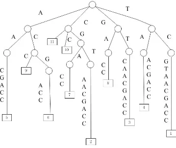
2.13 The suffix tree for the string TCGTAACGACC; . . . 14
2.14 The suffix array (SA) for the string TCGTAACGACC; . . . 15
2.15 Burrows-Wheeler transform for the string “ˆBANANA|”. . . 16
2.16 FM-index table for the string “acaacg$” via the Burrows-Wheeler matrix 17 2.17 Steps to match the substring “aac” in the string “acaacg$” [13]. . . . 17
2.18 Uniqueness scoring function [7] (exemplified by Mus musculus,
chr17:3028401-3028500). The minimum unique prefixes for each window are
illus-trated in the sequences shown. In each window of a fixed length,
counting the number of minimum unique substrings helps calculating
the uniqueness score. The minimum unique substrings, which are
indi-cated by stars, are used to add to the uniqueness score. The uniqueness
scores for the six windows shown are 7, 9, 7, 4, 1, 0, respectively. . . 19
2.19 Probe selection algorithm [7]. . . 20
2.20 The problem of sequence similarity in tiling genomic DNA [3]. . . 22
2.21 Multiple Feature Tiling [3]. Overlapping tiles using fractional offset
(e.g., one 25-mer probe placed every 5 nucleotides) and single-base
offset placement. . . 23
3.1 BLAST will extend the consecutive matches to find more similarities. 27
3.2 Comparison between non-spaced and spaced seeds. . . 27
3.3 Comparing sensitivity of space seed and BLAST seed [10]. . . 28
3.4 The overlap-allowed oligos and the non-overlapping oligos in a genome. 29
3.5 GC-content evaluation process. . . 31
3.6 The set of multiple spaced seeds used in the homology search phase. . 33
3.7 The process of similarity elimination. . . 35
3.8 The process of selecting oligonucleotides. . . 37
4.1 The set of multiple spaced seeds used in the closest non-target
similar-ity evaluation. . . 41
4.2 Closest non-target identity distribution for theDrosophila melanogaster
dataset. . . 43
4.3 Closest non-target identity distribution for the T.reesei dataset. . . . 44
4.4 Closest non-target identity distribution for the Mus musculus dataset. 45
4.5 Closest non-target identity distribution for theDrosophila melanogaster
dataset; the region of 75-100% identity. . . 46
4.10 Closest non-target identity distribution for the Mus musculus dataset;
all identity levels (left) and 75-100% identity (right). . . 47
4.11 Melting temperature distribution for theDrosophila melanogaster dataset.
. . . 48
4.12 Melting temperature distribution for the T.reesei dataset. . . 49
4.13 Melting temperature distribution for the Mus musculus dataset. . . 50
4.14 GC content distribution for the Drosophila melanogaster dataset. . . 51
4.15 GC content distribution for the T.reesei dataset. . . 52
4.16 GC content distribution for the Mus musculus dataset. . . 53
4.17 Good Oligo Distance distribution for theDrosophila melanogaster dataset.
. . . 54
4.18 Good Oligo Distance distribution for the T.reesei dataset. . . 55
4.19 Good Oligo Distance distribution for the Mus musculus dataset. . . 56
List of Tables
3.1 Encoding of genome sequence . . . 30
3.2 Nearest-Neighbor parameters for DNA/DNA duplexes (SantaLucia [23]) . . . 33
4.1 Commom factors for Evaluation. . . 39
4.2 Input data sets used for evaluation. . . 40
4.3 Good oligos comparison for Drosophila melanogaster. . . 42
4.4 Good oligos comparison for Trichoderma reesei. . . 42
4.5 Good oligos comparison for Mus musculus. . . 42
4.6 Time and memory for the Drosophila melanogaster dataset. . . 57
4.7 Time and Memory for the Trichoderma reesei dataset. . . 57
4.8 Time and Memory for the Mus musculus dataset. . . 57
that allows identification, e.g., using fluorescence, thus permitting the detection of
their target. It is therefore essential that good oligos do not cross-hybridize with
non-target sequences. Oligonucleotides have many important applications including
PCR (polymerase chain reaction) amplification, microarrays, or FISH (fluorescence
in situ hybridization) probes.
While traditional microarrays are commonly used for measuring gene expression
levels by probing for sequences of known and predicted genes, high-density, whole
genome tiling arrays probe intensively for sequences that are known to exist in a
contiguous region. Whole genome tiling arrays have many advantages such that the
high reproducibility among arrays, unbiased and complete genomic coverage, multiple
and potential overlaps, and probes representing transcription factor binding regions.
There are several programs for designing whole genome tiling oligonucleotide
probes, such as ArrayDesign [7] and OligoTiler [3]. The main procedure of the
lead-ing programs for detectlead-ing cross-hybridization is based on several derivative tools of
the suffix array [17] and BLAST (Basic Local Alignment Search Tool) [2]. For this
reason, they are not able to produce results that are close to optimal since they
al-low oligonucleotides that are too similar with non-targets, thus enabling unwanted
cross-hybridization. In addition, they can not produce the maximum number of good
Chapter 1. Introduction 2
oligonucleotides, thus not being able to detect every unique fragment.
In order to design better oligonucleotides, we present a new program, BOND-tile,
which uses the method of spaced seed-based similarity search and employs multiple
spaced seeds [15] computed by SpEED [9]. The proposed BOND-tile algorithm is
designed to search the non-overlapping unique oligonuleotide probes for whole genome
tiling, considering factors such as:
• Oligo placement
• Similarity between an oligonucleotide and its non-target sequences
• Melting temperature
• GC-content
• Heuristic oligo selection
The new BOND-tile program designs 100% good oligonucleotides without any
noisy output, and finds the largest number of unique oligonucleotides. It produces
significantly better oligonucleotides as shown by extensive comparison with leading
programs.
The thesis is organized as follows. After a brief introduction of the biological
background and computer science methods in Chapter 2, we describe completely
the new BOND-tile algorithm in Chapter 3, and perform the comparison against
ArrayDesign and OligoTiler in Chapter 4, concluding with a brief discussion of the
The second section explains the concept of oligonucleotides and their applications.
Finally, the central problem of the thesis, whole genome tiling, is introduced, together
with some of the leading programs for solving it.
2.1
Molecular biology primer
In order to understand the concepts of the thesis, we present a brief introduction to
basic biological background.
2.1.1
Organisms and cells
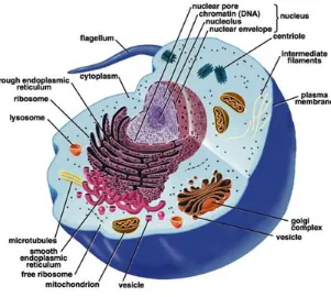
Every organism, a living system, is composed of cells. A cell is the functional unit
and basic structure of organisms. Organisms are classifed into unicellular and
multi-cellular. Cells have two types, eukaryotic and prokaryotic. Prokaryotic cells can live
independently, while eukaryotic cells are components of multicellular organisms. The
most important difference between eukaryotic and prokaryotic cells is that eukaryotic
cells include their organelles which are divided and wrapped by their membrane. The
organelles are the main site of occurring specific metabolic activities. Cells exchange
Chapter 2. Genome Tiling 4
information and make decisions through complex networks of chemical interaction
which are called pathways [1].
Figure 2.1: An eukaryotic cell. (from Wikipedia)
2.1.2
DNA, RNA, and proteins
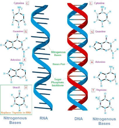
DNA, deoxyribonucleic acid (Fig. 2.2), is a biological macromolecule that contains
the genetic instructions to guide biological development and vital functions. The four
bases found in DNA are adenine (A), cytosine (C), guanine (G) and thymine (T).
RNA,ribonucleic acid (Fig. 2.2), is also a biological macromolecule which is
con-structed from nucleotides and chemically similar to DNA. The four bases found in
RNA are adenine (A), cytosine (C), guanine (G), and uracil (U). In the cell,
accord-ing to the different structures and functions, RNA is classified into three categories,
namely tRNA, rRNA, and mRNA. mRNA is the template of protein synthesis based
on translation from a DNA sequence; tRNA identifies the genetic code on the mRNA
and is the amino acid transporter; rRNA is contained in the ribosome which is the
Figure 2.2: Structure of DNA and RNA.
(http://chemistry.tutorvista.com/biochemistry/nucleic-acids.html)
Proteins are biological molecules composed of amino acids. They are the
func-tional molecules of the cell and can be classifed into groups such as structural proteins,
enzymes and transmembrane proteins. Biochemists often identify four distinct
as-pects of a protein’s structure (presented in Figure 2.3): primary structure, secondary
Chapter 2. Genome Tiling 6
Figure 2.3: Structure of proteins.
(http://www.entrenandotualimentacion.es/2013/07/03/suplementacion-con-whey-protein-en-ancianos/)
2.1.3
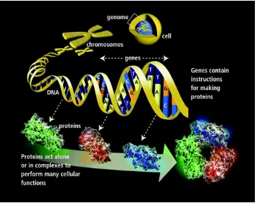
Genome, chromosome, and gene
The genome of an organism includes a complete set of DNA sequences. The DNA is
packaged into thread-like structures called chromosomes.
A gene is a piece of DNA that carries genetic information. The process of forming
proteins is guided by genetic information. Genes are the basic units of heredity to
control the characters of an organism.
The relationship between genome, chromosomes and genes is shown in Figure 2.4:
2.1.4
Thermodynamics of DNA
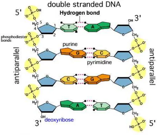
DNA is normally a double stranded macromolecule. The strands are held together by
Figure 2.4: Relationship of genome, chromosome and genes
The genome (inside the cell) contains all of an organism’s genetic instructions. (http://www.broadinstitute.org/blog/word-day-genome)
by binding two complementary DNA sequences together. This phenomenon is called
hybridization. Double-stranded DNA can be separated into two single strands by
heating. This process is called DNA melting. During the melting of DNA,
hydro-gen bonds between complementary bases will be broken. The melting temperature,
Tm, indicates the temperature at which the number of single-stranded molecules and
double-stranded molecules is the same.
In DNA, the pairs A=T have two hydrogen bonds, while C≡G have three hydrogen
bonds (Fig. 2.6). Therefore, C≡G is stronger than A=T. The GC content is the
percentage of C≡G pairs in DNA. Limits imposed on the GC content constrain the
range of melting temperature. Generally, sequences with a higher percentage of GC
base pairs have a higher Tm than AT-rich sequences do.
Several methods are available to calculate the melting temperature. The Nearest
Chapter 2. Genome Tiling 8
Figure 2.5: Double-stranded DNA. (from City University of New York) The 5’ end and the 3’ end refer to the two distinctive ends of DNA.
Figure 2.6: Hydrogen bonds between AT and GC base pairs. (from Wikipedia)
in detail in Chapter 3.
2.2
Oligonucleotides and applications
2.2.1
Oligonucleotides
A DNA oligonucleotide, abbreviated oligo, is a single-stranded chain of DNA that
is designed to bind uniquely to a target region (Fig. 2.7). A good oligo should not
Figure 2.7: An example of oligos hybridized with their target DNA sequences.
2.2.2
Applications of oligonucleotides
Oligo have many important applications, some of the most important ones of which
are listed below:
• PCR (polymerase chain reaction) amplification; oligos are used as primers whose
sequence is complementary to the 5’ end of the sequence targeted for
amplifi-cation.
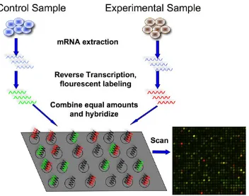
• Microarrays; these are collections of microscopic DNA spots attached to a solid
surface. The DNA sequences attached are the oligos. By specific target
hy-bridization, simultaneous measurement of the expression of large number of
genes is performed (Fig. 2.8).
• FISH (Fluorescence In Situ Hybridization) probes; oligos labelled with
fluores-cent dyes are used so that hybridization can be detected by fluorescence
mi-croscopy. This method can be used for detecting and localizing DNA or RNA
Chapter 2. Genome Tiling 10
Figure 2.8: A typical DNA microarray co-hybridization (2 dye) experiment. (http://bitesizebio.com/articles/introduction-to-dna-microarrays/)
2.3
Whole Genome Tiling
DNA microarrays are an effective technology commonly used for measuring gene
expression levels in biological and medical areas. Microarrays use one or several
probes for every gene. They probe for sequences of known and predicted genes.
Microarray chips have a branch referred to as tiling arrays. Instead of probing for
sequences of known or predicted genes that may be scattered throughout the genome,
whole-genome tiling arrays probe intensively for sequences that are known to exist
in a contiguous region (Fig. 2.9). In order to cover entire genomes, the density of
probes needs to be much higher than the traditional microarrays.
The significant advantages of tiling arrays over the traditional ones includes the
high reproducibility among arrays, unbiased and complete genomic coverage, multiple
and potential overlaps, and probes representing transcription factor binding regions
associa-Figure 2.9: Unbiased whole-genome tiling array designs [18].
Probes may be partially overlapping or nonoverlapping and tiled end to end.
tion studies for detection of genetic variants.
There are several approaches, presented in Figure 2.10, using whole-genome
high-density oligonucleotide tiling arrays for transcriptome characterization and genome
analysis.
Chapter 2. Genome Tiling 12
2.4
Sequence alignments
We present in the following sections two notions from computer science that are
necessary for understanding some of the whole genome tiling approaches. Sequence
alignment is a method widely used for comparing strings in order to find regions of
high similarity between them. Evolutionary related sequences have regions of high
similarity which show the structural and functional relationship between them.
Alignments are of two types: global and local. A global alignment is an alignment
in which every element in the two sequences is involved. A local alignment finds
similar regions (substrings) between the two sequences.
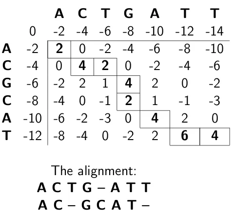
An earlier global alignment algorithm, based on dynamic programming, was
de-veloped by the Needleman and Wunsch [19]. An example is shown in Figure 2.11.
A
C
T
G
A
T
T
0
-2 -4 -6 -8 -10 -12 -14
A
-2
2
0
-2 -4
-6
-8
-10
C
-4
0
4
2
0
-2
-4
-6
G
-6
-2
2
1
4
2
0
-2
C
-8
-4
0
-1
2
1
-1
-3
A
-10 -6 -2 -3
0
4
2
0
T
-12 -8 -4
0
-2
2
6
4
The alignment:
A C T G – A T T
A C – G C A T –
Figure 2.11: Needleman-Wunsch alignment of two sequences; the dynamic programming matrix and the optimal alignment.
The Needleman-Wunsch algorithm may miss short but highly similar regions
There-G C C C T A
G C G
0
0
0
0
0
0
0
0
0
0
G
0
1
0
0
0
0
0
1
0
1
C
0
0
2
1
1
0
0
0
2
0
G
0
1
0
1
0
0
0
1
0
3
C
0
0
2
1
2
0
0
0
2
1
A
0
0
0
1
0
1
1
0
0
1
A
0
0
0
0
0
0
2
0
0
0
The alignment:
G C G
G C G
Figure 2.12: Smith-Waterman alignment of two sequences; the dynamic programming matrix and the best local alignment.
2.5
Text indexing
Text indexing is the general procedure of constructing a data structure from a given
text such that certain operations can be performed efficiently. The best known text
indexes are the suffix tree [26] and the suffix array [17].
The suffix tree of a string is a tree whose edges are labelled with substrings such
that every suffix of the string corresponds to a unique path from the root to a leaf.
Chapter 2. Genome Tiling 14
difficult. An example of a suffix tree is shown in Figure 2.13.
Figure 2.13: The suffix tree for the string TCGTAACGACC;
the leaves are labelled by the starting positions of the corresponding suffixes.
The suffix array (SA) of a string is defined as an array of positions sorted in the
lexicographical order of the corresponding suffixes of the string. The longest common
prefix (LCP) of two consecutive suffixes in the suffix array stores the length of the
longest shared prefix. Figures 2.14 gives an example of a suffix array and a LCP
array.
2.6
FM-index
The FM-index [5] is a compressed full-text substring index referring to an
10 4 TAACGACC 0
11 1 TCGTAACGACC 1
Figure 2.14: The suffix array (SA) for the string TCGTAACGACC; the third column gives the suffixes and the last the LCP array.
2.6.1
Burrows-Wheeler transform
The Burrows-Wheeler transform (BWT) is an algorithm applied in data compression.
The algorithm was invented by Michael Burrows and David Wheeler [4]. It transforms
a string of characters into a permutation of similar characters. When using this
method to convert a string, the algorithm only changes the order of the characters in
the string without changing any value of its characters. If the original string contains
some substrings that appear several times, then there will be several continuously
repeated characters on the transformed string, which would benefit compression.
BWT includes the following steps in order to implement the transformation:
• Create a table whose rows are all possible rotations of the string.
• Sort all rows in lexicographical order.
• Extract the last column of the table as the output.
The output contains some consecutive repeated characters so that it is easier to
compress. In addition, this transformation can be reversed without any additional
data being stored. Therefore, the BWT improves the efficiency of text compression
Chapter 2. Genome Tiling 16
Figure 2.15: Burrows-Wheeler transform for the string “ˆBANANA|”.
The string “ ˆBANANA|” is transformed into “BNN ˆAA| A” (the red vertical bar
indicates the ‘end of file’ pointer). (from Wikipedia)
2.6.2
The FM-index
The FM-index uses the Burrows-Wheeler transform along with the Suffix Array data
structure such that it allows compression of the input string, simultaneously
permit-ting fast substring queries. The most important advantage of the FM index is that
it uses significantly less space compared with the suffix array.
An example of how the FM-index finds the position of a substring without
un-compressing is shown in the following steps:
- Transforming the string “acaacg$” into the BWT string “gc$aaac” through
Burrows-Wheeler matrix of the string (the $ indicates the ‘end of file’ pointer),
synchronously recording the corresponding suffix array (Fig. 2.16).
- The substring “aac” is searched for using the BWT string and the alphabetical
order row. The pairs of continuing arrows indicate the region of the BWT
that includes all positions that correspond to the current suffix of the substring
Figure 2.16: FM-index table for the string “acaacg$” via the Burrows-Wheeler matrix that contains all rotations of the string sorted lexicographically. The 7th column gives the BWT output string and the last records the corresponding SA.
Figure 2.17: Steps to match the substring “aac” in the string “acaacg$” [13].
2.7
Leading programs for genome tiling
A significant amount of research has been performed for designing tiling
oligonu-cleotide probes. In this chapter, we present the top two current algorithms for whole
Chapter 2. Genome Tiling 18
2.7.1
ArrayDesign
ArrayDesign [7] constructs whole genome tiling arrays by defining a measure of
qual-ity for oligonucleotide probes named the uniqueness score (U). It is shown that U
is equivalent to the number of shortest unique substrings in the probe. A greedy
algorithm is given to design whole genome tiling arrays using probes that maximize
U. The outline of the ArrayDesign algorithm is as follows:
Defining the uniqueness score
To determine the uniqueness score, the minimum unique prefixes are computed at all
possible positions. This is reduced to a congruent relationship between the minimum
unique substrings and the distinct end positions of minimum unique prefixes (Fig.
2.18). The relationship is that counting the distinct end positions of minimum unique
prefixes helps computing the number of minimum unique substrings. In Figure 2.18,
the sequence of each minimum unique prefix in the windows is shown. Computing the
number of minimum unique substrings gives the uniqueness score for every window
of a fixed length.
Computing minimum unique prefixes
ArrayDesign uses an algorithm based on a simple technique to compute minimum
unique prefixes. The uniqueness problem involves the comparison of a huge number of
uniqueness queries against the same data set. A solution based on the FM-index was
developed. ArrayDesign first constructs the Burrows-Wheeler transform, then uses a
multiway merging procedure which synchronously reads all suffix arrays [17] from left
to right. After each merging step, the next suffix is acquired in the sorted order of
all suffixes and obtain the corresponding character of the Burrows-Wheeler transform
and the other related information. After the FM-index is stored, the uniqueness
Figure 2.18: Uniqueness scoring function [7] (exemplified by Mus musculus, chr17:3028401-3028500). The minimum unique prefixes for each window are illus-trated in the sequences shown. In each window of a fixed length, counting the number of minimum unique substrings helps calculating the uniqueness score. The minimum unique substrings, which are indicated by stars, are used to add to the uniqueness score. The uniqueness scores for the six windows shown are 7, 9, 7, 4, 1, 0, respec-tively.
Validating the uniqueness score
A collection of 50-mer probes from the NimbleGen whole genome tiling array was
used to validate the uniqueness score. For each of these probes, the uniqueness score
is determined as explained above and the number of hybridization-quality alignments
for each probe to the genome is computed using BLAT [12] (BLAST-Like Alignment
Tool).
Probe selection algorithm
The optimal probes are calculated (as shown in Figure 2.18) using a greedy
Chapter 2. Genome Tiling 20
Figure 2.19 illustrates the process of the probe selection algorithm.
Figure 2.19: Probe selection algorithm [7].
The parameters that are considered in the probe selection step are:
• Making sure not to include any specific runs which produce unsatisfactory
oligonucleotides (e.g., more than 6 consecutive G’s).
• Checking that the fragment can only contain less than a pre-set percentage
of palindromic sequence to eliminate probes with significant self-hybridization
potential.
• Choosing the probes with less than a given maskless array synthesis (MAS)
manufacturing cycle limit.
2.7.2
OligoTiler
OligoTiler [3] determines the similarity degree of many oligonucleotide sequences from
large genomes. It gives two algorithms for finding an optimal tile path. The first,
implemented by a dynamic programming approach, finds the optimal tiling in linear
time and space and the second uses a heuristic search to decrease the space
complex-ity to satisfy a constant requirement. The main methods and considered factors of
OligoTiler are shown below.
Sequence similarity and single-copy tiling
This design of tiling arrays involves computing the degree of similarity of any given
oligonucleotide sequence in a large genome in order to generate a single-copy tile
path which is represented on the array (Fig. 2.20). This intends to identify and
Chapter 2. Genome Tiling 22
elsewhere in the genome. Due to the problem of memory constraints and sequence
mismatches, OligoTiler uses a BLAST-like scheme.
Figure 2.20: The problem of sequence similarity in tiling genomic DNA [3].
(A) Calculating the level of similarity (shown by the grey bars). The sequences
are eliminated from the tiling path when the sequence redundancy surpasses the pre-set threshold (shown by the dashline). (B) Avoiding redundant or repetitive sequence, simultaneously retaining sufficient sequence tiling. (C) With the minimum tile connecting with their contiguous tile, the level of non-repetitive sequence coverage decreases. (D) The tiling algorithms is enabled to involve a few redundant sequences in an optimal fashion aiming at acquiring a higher percentage of non-repetitive DNA.
Repeat identification and low-complexity filtering
On a global scale, OligoTiler adopts libraries of known repeats identified in
ge-nomic DNA through comparison of sequences using BLAST [2] (Basic Local
Align-ment Search Tool). Using software such as RepeatMasker (http://ftp.genome.
washington.edu/RM/RepeatMasker.html) is the most convenient way to accomplish
it.
Tiling resolution
An important factor, tiling resolution, involves determining how to subdivide the
rep-Figure 2.21: Multiple Feature Tiling [3]. Overlapping tiles using fractional offset (e.g., one 25-mer probe placed every 5 nucleotides) and single-base offset placement.
Thermodynamic properties of oligonucleotide probes
One of the factors of OligoTiler in selecting oligonucleotide sequences for tiling arrays
is the predicted hybridization affinity [23]. For sequences over thirteen nucleotides,
hybridization affinity is almost the equivalent of calculating the melting temperature
using this formula:
Tm = 64.9 + 41×(nG+nC −16.4)/(nA+nT +nG+nC) (2.2)
wheren[A,C,G,T] denotes the number of each nucleotide in the DNA sequence.
Chapter 2. Genome Tiling 24
sequence [21]:
Tm = [∆H(kcal/◦C×M ol)/∆S+R×ln([oligo]/2)]−273.15◦C (2.3)
In order to increase the consistency ofTmwhich corresponds to each probe, computing
the melting temperature helps shifting the replacement of oligonucleotide within every
non-repetitive region. OligoTiler selects the individual probe from each available
region such that its computed Tm is closer to the optimal temperature than the
unsatisfactory region. The universal set of oligos can be shifted all together so that
their aggregate Tm can be optimized.
Additional Parameters
Other parameters considered to create oligonucleotides can be set by the user:
• “IR region” considers how OligoTiler deals with the potential inverted repeats
at the two ends of an oligo. It gives a limit of how many characters at the two
ends should be checked in order to avoid inverted repeats.
• “IR require” considers the same parts as above. It means the number of
match-ing base pairs that must be checked within the “IR region” such that the start
Then, we introduce the notion of spaced seeds, that is central to our new design.
3.1
Problems with previous designs
Two leading programs for whole genome tiling arrays were described in the last section
of Chapter 2. We point out several problems with their design, common to all existing
tools, not just the two we have described.
The first, and most important problem, is hybridization with non-targets. DNA
hybridization happens between complementary sequences. However, the
complemen-tarity does not have to be perfect for strong hybridization to take place. Since oligos
are supposed to bind only to their targets, their complementary sequences must be
very different from any non-target sequence. The identity percentage denotes the
percentage of matches between two sequences. Usually, identity of 75% or lower is
required in order to prevent binding to non-targets [11]. Differently put, the identity
between the complement of the oligo and any non-target must be less than 75%.
The existing programs succeed only partially at achieving this goal. Some use
various heuristics, with limited success, others use BLAST [2] in order to find
simi-larities and eliminate them. BLAST however has limitations in finding simisimi-larities.
Chapter 3. BOND-tile 26
For instance, BLAST finds only 40% of the similarities of length 50 and identity 75%.
Its sensitivity is shown as the pink line in Figure 3.3.
The second problem is that the current programs do not find the highest possible
number of oligos, as it will be seen in our evaluation.
Third, the methods used in evaluating these programs suffer from the same
prob-lem of not being able to thoroughly look for similarities. For example, the survey [14]
uses BLAST which, as we indicated above, is inappropriate.
These problems appear also in programs designing traditional oligonucleotides
and they were corrected by the recent BOND program [10] (BOND stands for Basic
OligoNucleotide Design). Using the same method, of spaced seed-based similarity
search, we extend here the BOND program to solve the more difficult problem of
whole genome tiling. Our new program is called BOND-tile.
3.2
Spaced seeds
A full alignment procedure, the dynamic programming algorithm of Smith-Waterman,
was used before fast algorithms were developed. The Smith-Waterman algorithm has
perfect sensitivity but its quadratic time complexity makes it impossible to apply
for large sequences. Hence, heuristics approaches that can identify similarity fast are
needed. The Basic Local Alignment Search Tool [2], BLAST, became the most widely
used algorithm in searching similarities. It is assumed that high similarity implies
sharing a long substring which results in local alignment of the two sequences. The
development of BLAST was based on this idea. BLAST uses a consecutive seed
11111111111 to select 11 consecutive positions which are identical. A ’1’ denotes a
match. The 11 consecutive matches are called a hit. BLAST finds pairs of such
matching strings (hits) and then attempts to extend the similarity both ways (Fig.
3.1). Consecutive matches are easy to find, but BLAST may miss some high similarity
regions with a few mismatches. (As an example, one can imagine a similarity where
all positions match, except for every eleventh one. The similarity is about 91%, yet
PatternHunter [16] presented a homology search algorithm by using an
non-consecutive spaced seed to check matches between sequences, which has a higher
sensitivity. PatternHunter’s seed is 111*1**1*1**11*111; a ‘1’ denotes a match and
‘*’ represents a “don’t care” position. In other words, it only checks the positions
directly corresponding to 1’s, while ignoring the positions corresponding to *’s. The
weight of a seed refers to the number of 1’s. The total number of 1’s and *’s is the
length of a seed. The probability of a hit depends only on the weight of the seed. So,
between non-spaced and spaced seeds with the same weight, the expected number of
hits is the same. Spaced matches have higher sensitivity because of less overlapping
between hits. Put another way, with the shifting of a seed, spaced seeds need more
matches to detect another hit. Therefore, consecutive seeds suffer from hit clustering
and thus spaced seeds can detect more similarities. Figure 3.2 illustrates the
compar-ison between non-spaced and spaced seeds.
Figure 3.2: Comparison between non-spaced and spaced seeds.
A hit of the contiguous seed (left) requires only one more match for another hit at the next position, whereas for the spaced seed (right) six additional matches are needed.
ap-Chapter 3. BOND-tile 28
plied together for homology searching, which is called multiple spaced seeds. Using
multiple seeds can reach almost perfect sensitivity [15]. To design an efficient
simi-larity check, we need optimal multiple spaced seeds but they are hard to compute.
Several heuristic algorithms have been designed to calculate multiple spaced seeds,
but all of them have exponential time complexity except SpEED [9, 8]. This
al-gorithm calculates highly sensitive multiple spaced seeds and was used to compute
the seeds employed by BOND-tile. Figure 3.3 illustrate the comparison of BLAST’s
seed and multiple spaced seeds computed by SpEED which was used by the BOND
program for designing oligos.
Figure 3.3: Comparing sensitivity of space seed and BLAST seed [10].
The green line shows weight 6 multiple spaced seeds; the blue line shows weight 9 multiple spaced seeds; the pink line shows the BLAST seed;
3.3
The BOND-tile algorithm
In this section, we explain in detail the BOND-tile algorithm for designing
two approaches. We choose the latter method to design BOND-tile as it produces
better results. The two methods are described below:
- The overlap-allowed oligos can start from every position of their window in the
whole genome such that the oligos in consecutive windows may overlap. Put
another way, the start position of an oligo may happen within the previous
oligo.
- The non-overlapping oligos are defined such that consecutive oligos have no
overlap. Every oligo is fully contained in its target window. This method is
named EasyCut.
Chapter 3. BOND-tile 30
Outline of BOND-tile
The proposed BOND-tile algorithm is designed to search non-overlapping unique
oligonuleotide probes from each contiguous window (EasyCut).
BOND-tile marks every position in the genome as a possible candidate or not for
an oligo ending at that position. Every step deals only with candidate regions in the
genome. Once a position is marked as non-candidate, the remaining steps will not
consider it.
Then main steps of BOND-tile are presented below.
• Encoding the input sequences
• Fast elimination of high-similarity (spaced seed-based)
• GC-content management
• Melting temperature evaluation
• Intensive elimination by homology search (spaced seed-based)
• Final oligo extraction
Every step of the algorithm is explained in detail in the following subsections.
3.3.2
DNA encoding
BOND-tile encodes the input sequences in binary code, using two bits per nucleotide
(see Table 3.1).
Table 3.1: Encoding of genome sequence
Nucleotide base Binary encoding
A 00
C 01
G 10
32 nucleotide bases each time.
Also, it saves three quarters of the memory usage. Encoding each base requires
only two bits, while, in regular storage, every nucleotide base needs one byte due to
the character data type. This is helpful and efficient in managing large genomes.
3.3.3
GC content
GC-content refers to the proportion of G (guanine) and C (cytosine) in a DNA
se-quence. The genome of one organism, or specific segments of DNA and RNA, has
specific GC-content. To evaluate the GC-content, we developed an algorithm which
determines the thresholds of the minimum and maximum GC-content through a
user-defined schema. In the proposed algorithm, the default values are set as 30% and
70% respectively. It can be reset by the user.
Chapter 3. BOND-tile 32
It can be seen from Figure 3.5 that the management of GC-content is conducted
from the right end of the encoded genome, screening to the left end. Among the whole
procedure, the percentage of guanine and cytosine will be examined; meanwhile some
oligo candidate positions whose GC-content percentage is outside the predefined range
will be eliminated. Every end position of eliminated subsequences will be marked as
non-candidate.
3.3.4
Melting temperature
The melting temperature, Tm, is one of the key parameters for designing the oligo
probes. To maximise uniformity for the obtained oligonucleotide set, melting
temper-atures of oligonucleotides need to differ only slightly. The Nearest Neighbour model
is the most widely used approach to calculate the melting temperature by applying
it with the parameters from SantaLucia [23] or Rychlik [20]. BOND-tile uses this
approach to compute theTm[6, 24]:
Tm =
∆H
Rln(C/4) + ∆S−273.15 + 12log[Na
+] (3.1)
where ∆H, enthalpy(k.cal/mol), denotes the total energy exchange between the
sys-tem and its surrounding environment, the ideal gas constant is denoted by R =
1.987 (cal/mol.K), C denotes the molar concentration of oligo sequence, ∆S,
en-tropy(cal/mol.K), is the energy spent to achieve self-organization by the system, and
[Na+] represents the molar concentration of salt. The values of ∆H and ∆S are
presented in Table 3.2.
The melting temperature of the candidate at every position will be computed
and stored. The ones falling outside the user defined range are considered as
GA/CT -8.2 -22.2
CG/GC -10.6 -27.2
GC/CG -9.8 -24.4
GG/CC -8.0 -19.9
Init. w/term. G/C 0.1 -2.8
Init. w/term. 2.3 4.1
A/T Symmetry correction 0 -1.4
3.3.5
Similarity search
The spaced seed-based similarity search involves finding and investigating all hits
corresponding to all spaced seeds. This can be a time consuming task and, in order
to speed up the process, we shall perform the search in two phases. In the first phase,
for each seed, only one position of each hit is considered. This helps eliminating
vary fast large regions of high similarity. In the second phase, all possible hits are
considered, thus using the full power of the seeds.
BOND-tile employs the set of eight multiple spaced seeds of weight 10 shown in
Figure 3.6. These seeds are selected bySpEED [9, 8].
111*1**11*1*111
11**1*1**1***1***11*11 1111***1***1****11*1*1 11**11****1*1***1*11*1 111**1***1**1**1****111 11*1**1*******1*1**1***111 11*1***1****1*****1***1**111 11*1*1*****1*****1*****11*11
Chapter 3. BOND-tile 34
Hash table construction
Given a spaced seed s, an s-mer is a sequence of symbols that contains nucleotides for the 1-positions and zeros for the∗-positions. For example, ifs= 11*1**1, then an example of ans-mer is AC0G00T. The don’t care positions ‘∗’ are ignored by having 0’s in those places. A hit is given by a pair of identicals-mers. Therefore, we store alls-mers of each seed in a hash table. Since the nucleotides are encoded in binary, thes-mers are simply sequences of bits. To enable fast computation, we use a bitwise AND between the seed and the DNA sequences. The seed is suitably encoded by 1
→11, ∗ →00.
A hash table is created for each of the eight spaced seeds. Linear probing is used
for handling hash collisions. The algorithm checks the bases starting from the right
end of the encoded genome and slides to the left end. The s-mer’s integer value of
each position in the genome will be searched by using the seed model. If found, a hit
is discovered and investigated for potential similarity.
Phase I: Fast elimination
In the fast elimination phase, BOND-tile looks quickly for the potentially
unsatisfac-tory oligo positions, and eliminates them after finding high-similarity regions.
BOND-tile calculates thes-mer integer value of each position in the genome, then searches the hash table for its hash value. If the corresponding hash value does not
exist in the hash table, the BOND-tile algorithm uses this hash value to be the hash
key and inserts the related position into the hash table. In the case that the hash
value already exists in the hash table, that means a ‘hit’ is found.
After finding a hit, BOND-tile extends the matches corresponding to the hit both
left and right as long as the similarity level of the two regions is above the
user-specified threshold. BOND-tile eliminates positions of the two regions by marking
them as non-candidates. Figure 3.7 shows how the extension works. The default
Figure 3.7: The process of similarity elimination.
Phase II: Intensive search and elimination
In the intensive elimination phase, BOND-tile first calculates thes-mer integer value of each position, and inserts this integer value as a hash key and synchronously input
all the related positions into the hash table. In case the obtained integer value can
be found as a hash key, only the related position will be put into the position array
which corresponds to this hash key.
After all the hash tables are completely created, the algorithm will scan every
candidate position in each window using a heuristic that tried the more likely ones
first (details in Section 3.3.6). For each position considered, all hits of all s-mers corresponding to all eight seeds are investigated. That is why this phase is called
intensive.
Differrence between fast and intensive elimination
To clarify, in the fast searching stage, only one position for each corresponding hash
Chapter 3. BOND-tile 36
last occurrence of the corresponding hit. In the intensive elimination, all candidate
positions and their corresponding hash values are kept in the hash table to be prepared
for similarity check. In addition, in every oligo candidate, the s-mer integer of every position will be used to search for similarity.
3.3.6
Oligonucleotide selection
In the selection phase, BOND-tile subdivides the genome into a large number of
contiguous windows of a fixed length. The purpose is to select non-overlapping
(EasyCut) unique oligonuleotide probes from each window. BOND-tile checks
each tiling window to eliminate all unsatisfactory sequences and select the unique
oligonuleotide probes.
Recall that BOND-tile stores every position in the genome, whether it is a
candi-date or not. To obtain the maximum number of unique oligo probes, the algorithm
will execute all steps by checking every possible position in each tiling window. In
ad-dition, to maintain high quality of oligo probes as well as good speed, before running
the search step of intensive elimination, BOND-tile chooses the middle position of a
region of consecutive candidates, since it is expected to have the lowest similarity with
any other region. For example, if the length of one region of consecutive candidates
is l and the end position of this region is j, the priority selected position is j - l/2. The process is shown in Figure 3.8.
As shown in the upper part of Figure 3.8, there are several candidate sequences
(green lines) and non-candidate sequences (red lines). The end positions of those
sequences are marked as green ticks and red crosses. The longest region of consecutive
green ticks, which means the longest region of consecutive candidates, is chosen to
be considered. In the lower part, the end position of the considered region is j and
the length of the region is l. Then the first picked candidate we try is shown in the
green box. Its end position isj - l/2. After selecting the preferred candidate, we use intensive elimination phase to verify that it is a good oligo. When an oligo is found
Chapter 4
Evaluation
This chapter presents the evaluation of experimental results. We compare the
per-formance of the BOND-tile algorithm with two leading programs for designing whole
genome tiling arrays, ArrayDesign [7] and OligoTiler [3].
4.1
General setup
After implementing the whole genome tiling program, BOND-tile, several evaluation
programs focusing on assessing the performance of BOND-tile were written as well.
In this chapter we evaluate the computational results of ArrayDesign, OligoTiler and
BOND-tile by comparing them according to the following factors:
- Identity with closest non-target (similarity check),
- Melting temperature,
- GC-content,
- Distance between consecutive oligos,
- Time,
- Space.
In all plots shown in this chapter, blue parts denote the results of ArrayDesign,
purple (light or dark) parts denote OligoTiler’s and green denote BOND-tile’s.
Defined Value
Parameters ArrayDesign OligoTiler BOND-tile
Oligo length 60bp 60bp 60bp
Window size 150bp 150bp 150bp
Overlapping allowed No(EasyCut) Very little (default, web) No(EasyCut)
GC content No Limit N/A No Limit
Melting temp No Limit N/A No Limit
Secondary structure No Limit IRregion=0 IRrequire=0 Turned Off
Everything else Default Values Default Values Default Values
4.2
Datasets
We use the following data sets as our input files. The FASTA file of Drosophila
melanogaster DNA chromosome 2L is downloaded from the pdf site: ftp://ftp.
ensembl.org/pub/release-67/fasta/drosophila_melanogaster/dna. The unmasked
FASTA file of Trichoderma reesei genome v.2.0 is downloaded from the
Depart-ment of Energy Joint Genome Institute website (JGI): http://genome.jgi-psf.
org/Trire2/Trire2.home.html. We also use NCBI Build 36 of the Mus musculus
DNA chromosome 17 downloaded from release 40 of Ensembl (ftp://ftp.ensembl.
org/pub/release-40/mus_musculus_40_36a/data/fasta/dna/). The information
Chapter 4. Evaluation 40
Table 4.2: Input data sets used for evaluation.
Species model Genome size Chromosome Description
Drosophila melanogaster
23011544 bp 2L Drosophila
melanogaster BDGP5 67 dna chromosome 2L Trichoderma
reesei
33454791 bp All Trichoderma
reeseiV2
Assem-bledScaffolds
Mus musculus 95177420 bp 17 Mus musculus
NCBIM36 40
dna chromosome 17
4.3
Operation Environment
The proposed algorithm is implemented in C++, and parallelized using openMP.
All computations were performed on the SHARCNET (Shared Hierarchical
Aca-demic Research Computing Network) which is a high performance computing
con-sortium. We used some nodes of the “shadowfax” cluster whose characteristics are
given below:
• Processor: Intel Xeon E6-2620 @ 2.0GHz, 2 sockets, 12 cores
• RAM: 256GB
• Operating System: Linux version CentOS 6.3
(see Fig. 4.1). The seeds were also computed using SpEED [9]. Their sensitivity is
shown by the green curve in Figure 3.3.
111*1*11 11**1**111 11*1*****1*11 1*1***1****111 1*1**1**1***1*1 11***1****1**1*1 11*1******1***1*1 11******1****1**11
Figure 4.1: The set of multiple spaced seeds used in the closest non-target similarity evaluation.
If an oligo probe has more than 75% similarity with non-target regions, we mark
it as a bad oligo, otherwise it is considered good. The evaluation program runs fairly
slow because we use the multiple spaced seeds of weight six so that the evaluation
program has high sensitivity, which results in a large number of hits.
The experimental results are shown in Tables 4.3-4.5. The percentage of good
oligos computed by BOND-tile is 100%, while for the others, it varies between 70%
and 97%. In addition, BOND-tile always obtains more good oligos than the other two
programs. The difference is particularly big for the largest dataset where BOND-tile
Chapter 4. Evaluation 42
Table 4.3: Good oligos comparison for Drosophila melanogaster.
Algorithm Total Oligos Good Oligos % of Good Oligos
ArrayDesign 153409 143260 93.38
OligoTiler 153410 142457 92.86
BOND-Tile 144707 144707 100.00
Table 4.4: Good oligos comparison forTrichoderma reesei.
Algorithm Total Oligos Good Oligos % of Good Oligos
ArrayDesign 222721 216736 97.31
OligoTiler 222793 215724 96.83
BOND-Tile 218319 218319 100.00
Table 4.5: Good oligos comparison for Mus musculus.
Algorithm Total Oligos Good Oligos % of Good Oligos
ArrayDesign 608461 462396 75.99
OligoTiler 608397 430023 70.68
BOND-Tile 499396 499396 100.00
The comparison for non-target similarity evaluation of ArrayDesign, OligoTiler
and BOND-tile is illustrated in Figures 4.2-4.10.
Figure 4.2-4.4 show the distribution of the oligos computed by the three programs
with respect to the percentages identity with the closest non-target. We show both
histograms and box-and-whiskers plots. BOND-tile has no oligos at identity higher
than 75%. For the largest dataset, the distribution of the oligos of BOND-tile is
significantly better than both the other programs (see Fig. 4.4, bottom). Also,
0
10000
%Identity
5356 606366 707376 808386 909396 100
0
10000
%Identity
5356 606366 707376 808386 909396 100
0
10000
%Identity 5356 606366 7073
ArrayDesign OligoTiler BOND−tile
50
60
70
80
90
100
Algorithms
%Identity
Closest non−target identity of oligos (Drosophila Mel. dataset)
Chapter 4. Evaluation 44
0
20000
40000
60000
Closest non−target identity of ArrayDesign oligos (T.reeseiV2 dataset)
%Identity
Oligos
555861 656871 757881 858891 9598
0 10000 20000 30000 40000 50000 60000 70000
Closest non−target identity of OligoTiler oligos (T.reeseiV2 dataset)
%Identity
Oligos
555861 656871 757881 858891 9598
0 10000 20000 30000 40000 50000 60000 70000
Closest non−target identity of BOND−tile oligos (T.reeseiV2 dataset)
%Identity
Oligos
555861 656871 75
ArrayDesign OligoTiler BOND−tile
50 60 70 80 90 100 Algorithms %Identity
Closest non−target identity of oligos (T.reeseiV2 dataset)
0
20000
40000
%Identity
555861 656871 757881 858891 9598
0
20000
%Identity
555861 656871 757881 858891 9598
0
20000
%Identity 555861 656871 75
ArrayDesign OligoTiler BOND−tile
50
60
70
80
90
100
Algorithms
%Identity
Closest non−target identity of oligos (Mus_musculus dataset)
Figure 4.4: Closest non-target identity distribution for the Mus musculus dataset.
The histograms for the identity between 75-100% are shown in Figures 4.5-4.7.
The same information is presented in the form of line graphs in Figures 4.8-4.10, this
Chapter 4. Evaluation 46 0 2000 4000 6000 8000
Closest non−target identity of ArrayDesign oligos (Drosophila Mel. dataset)
%Identity
Oligos
75 78 80 83 85 88 90 93 95 98 100
0
2000
4000
6000
8000
Closest non−target identity of OligoTiler oligos (Drosophila Mel. dataset)
%Identity
Oligos
75 78 80 83 85 88 90 93 95 98 100
0
2000
4000
6000
8000
Closest non−target identity of BOND−tile oligos (Drosophila Mel. dataset)
%Identity
Oligos
75
Figure 4.5: Closest non-target identity distribution for the Drosophila melanogaster dataset; the region of 75-100% identity.
0 200 400 600 800 1000
Closest non−target identity of ArrayDesign oligos (T.reeseiV2 dataset)
%Identity
Oligos
75 78 80 83 85 88 90 93 95 98 100
0 200 400 600 800 1000
Closest non−target identity of OligoTiler oligos (T.reeseiV2 dataset)
%Identity
Oligos
75 78 80 83 85 88 90 93 95 98 100
0 200 400 600 800 1000
Closest non−target identity of BOND−tile oligos (T.reeseiV2 dataset)
%Identity
Oligos
75
Figure 4.6: Closest non-target identity distribution for the T.reesei dataset; the
region of 75-100% identity.
0
10000
20000
30000
40000
Closest non−target identity of ArrayDesign oligos (Mus_musculus dataset)
%Identity
Oligos
75 78 80 83 85 88 90 93 95 98 100
0
10000
20000
30000
40000
Closest non−target identity of OligoTiler oligos (Mus_musculus dataset)
%Identity
Oligos
75 78 80 83 85 88 90 93 95 98 100
0
10000
20000
30000
40000
Closest non−target identity of BOND−tile oligos (Mus_musculus dataset)
%Identity
Oligos
75
Figure 4.7: Closest non-target identity distribution for the Mus musculus dataset;
Figure 4.8: Closest non-target identity distribution for the Drosophila melanogaster dataset; all identity levels (left) and 75-100% identity (right).
50 60 70 80 90 100
0 20000 40000 60000 80000 %Identity Oligos
Closest non−target identity of oligos (T.reeseiV2 dataset)
Algorithm BOND−tile ArrayDesign OligoTiler
75 80 85 90 95 100
0 200 400 600 800 1000 1200 %Identity Oligos
Closest non−target identity of oligos (T.reeseiV2 dataset)
Algorithm BOND−tile ArrayDesign OligoTiler
Figure 4.9: Closest non-target identity distribution for the T.reesei dataset; all
identity levels (left) and 75-100% identity (right).
50 60 70 80 90 100
0 50000 100000 150000 %Identity Oligos
Closest non−target identity of oligos (Mus_musculus dataset)
Algorithm BOND−tile ArrayDesign OligoTiler
75 80 85 90 95 100
0 10000 20000 30000 40000 %Identity Oligos
Closest non−target identity of oligos (Mus_musculus dataset)
Algorithm BOND−tile ArrayDesign OligoTiler
Figure 4.10: Closest non-target identity distribution for theMus musculus dataset;
Chapter 4. Evaluation 48
4.5
Melting temperature
As shown in Figures 4.11-4.13, the distribution of the melting temperature is fairly
similar among the three candidate programs.
0
50
100
150
Tm of ArrayDesign oligos (Drosophila Mel. dataset)
Tm(C degree)
Oligos
51.8457.22 62 65.7 70 73.778 81.786 89.8
0
50
100
150
Tm of OligoTiler oligos (Drosophila Mel. dataset)
Tm(C degree)
Oligos
49.5254.7 59 62.767 70.775 78.7 83 86.791.5
0 20 40 60 80 100 120 140
Tm of BOND−tile oligos (Drosophila Mel. dataset)
Tm(C degree)
Oligos
51.53 56.84 61 64.769 72.777 80.7 85 88.7
ArrayDesign OligoTiler BOND−tile
50 60 70 80 90 100 Algorithms Tm(C degree)
Melting temperature of oligos (Drosophila Mel. dataset)
Figure 4.11: Melting temperature distribution for the Drosophila melanogaster
0
50
100
Tm(C degree)
Oligos
53.05 576063666972757881848790 93.94
0
50
100
Tm(C degree)
Oligos
50.14 55.6606468 7276 808488 92.2
0
50
100
Tm(C degree)
Oligos
52.29 56.8 60.965687174778083868992
Chapter 4. Evaluation 50 0 100 200 300 400 500 600 700
Tm of ArrayDesign oligos (Mus_musculus dataset)
Tm(C degree)
Oligos
52.3158.46367 7175 7983 8791 95.4
0 100 200 300 400 500 600
Tm of OligoTiler oligos (Mus_musculus dataset)
Tm(C degree)
Oligos
48.8154 5862 6670 7478 8286 9094 99.35
0 100 200 300 400 500
Tm of BOND−tile oligos (Mus_musculus dataset)
Tm(C degree)
Oligos
53.55 5963 6771 7579 838791 95.5
0 2000 4000 6000 8000 GC content(%) Oligos
051016 23 3036 43 5056 63 7076 83
0 2000 4000 6000 8000 GC content(%) Oligos
051016 23 3036 43 5056 63 7076 83
0 2000 4000 6000 GC content(%) Oligos
051016 23 3036 43 5056 63 7076 83
ArrayDesign OligoTiler BOND−tile
0 20 40 60 80 100 Algorithms GC content(%)
GC content of oligos (Drosophila Mel. dataset)
Chapter 4. Evaluation 52
0
5000
10000
15000
GC content of ArrayDesign oligos (T.reeseiV2 dataset)
GC content(%)
Oligos
0510162228344046 53 6066 73 8086
0
5000
10000
15000
GC content of OligoTiler oligos (T.reeseiV2 dataset)
GC content(%)
Oligos
051016 23 3036 43 5056 63 7076 83
0
5000
10000
15000
GC content of BOND−tile oligos (T.reeseiV2 dataset)
GC content(%)
Oligos
051016 23 3036 43 5056 63 7076 83
ArrayDesign OligoTiler BOND−tile
0 20 40 60 80 100 Algorithms GC content(%)
GC content of oligos (T.reeseiV2 dataset)
0
10000
20000
GC content(%)
Oligos
051016 232935414753 6066 73 8086 93
0
10000
GC content(%)
Oligos
051016 23 3036 43 5056 63 7076 83 9096
0
5000
10000
15000
GC content(%)
Oligos
051016 23 3036 43 5056 63 7076 83 90
ArrayDesign OligoTiler BOND−tile
0
20
40
60
80
100
Algorithms
GC content(%)
GC content of oligos (Mus_musculus dataset)
Chapter 4. Evaluation 54
4.7
Distance between oligos
Figures 4.17-4.19 illustrate the distance, in base pairs, between the contiguous good
oligos. In other words, we eliminate all bad oligos produced by ArrayDesign and
Olig-oTiler before calculating the oligo distances. It can be seen that the oligo distance
parameter of BOND-tile is slightly better than OligoTiler and both are much better
than ArrayDesign. 0 500 1000 1500 2000 2500 3000
Distance of ArrayDesign oligos (Drosophila Mel. dataset)
Distance between good oligos(base)
Oligos
60 91 145 245 414 701 1256 24004722 9041 18328 70045
0 20000 40000 60000 80000 100000 120000 140000
Distance of OligoTiler oligos (Drosophila Mel. dataset)
Distance between good oligo(base)
Oligos
150 300 60010501950 3750 6600 12300 70050
0 20000 40000 60000 80000 100000 120000 140000
Distance of BOND−tile oligos (Drosophila Mel. dataset)
Distance between good oligo(base)
Oligos
65 96 150 247 407 675 1176 21994181 769415511 36727
ArrayDesign OligoTiler BOND−tile
5e+01 5e+02 5e+03 5e+04 Algorithms Distance betw
een good oligos(base)
Distance of good oligos (Drosophila Mel. dataset)
Figure 4.17: Good Oligo Distance distribution for the Drosophila melanogaster
Distance between good oligos(base) 60 79 108 153 217 307 435 618 876 12931999 30604794 10431
Distance between good oligos(base)
1 3 7 1629 4881 144 300580 1171 25505700 17914
Distance between good oligos(base)
62 80 108 150 209 291 405 563 784 11361733 2593 38976161 10414
ArrayDesign OligoTiler BOND−tile
1
10
100
1000
10000
Algorithms
Distance betw
een good oligos(base)
Distance of good oligos (T.reeseiV2 dataset)
Chapter 4. Evaluation 56
0
2000
4000
6000
8000
10000
Distance of ArrayDesign oligos (Mus_musculus dataset)
Distance between good oligos(base)
Oligos
60 93 152 264 458 794 1463 2867 5616 1175026883 59761 231835
0e+00
1e+05
2e+05
3e+05
Distance of OligoTiler oligos (Mus_musculus dataset)
Distance between good oligos(base)
Oligos
12 150298 579 1220 2725 6150 1485041045 116646
0
50000
100000
150000
200000
250000
300000
350000
Distance of BOND−tile oligos (Mus_musculus dataset)
Distance between good oligos(base)
Oligos
60 92 150 260 451 782 1440 2822 5533119822732665745 234564
slow, probably due to the very simple collision resolving scheme. (We did not have
time to try something else.)
Considering the fact that designing of tiling oligos is not done very often, all times
and memory requirements are perfectly acceptable.
Table 4.6: Time and memory for the Drosophila melanogaster dataset.
Algorithm Time(s) Memory(Mb) Total Oligos Good Oligos
ArrayDesign 3212 763.4 153409 143260
OligoTiler about 60 (web) 153410 142457
BOND-Tile 56 1731 144707 144707
Table 4.7: Time and Memory for the Trichoderma reesei dataset.
Algorithm Time(s) Memory(Mb) Total Oligos Good Oligos
ArrayDesign 4687 846.5 222721 216736
OligoTiler about 120 (web) 222793 215724
BOND-Tile 94 2252 218319 218319
Table 4.8: Time and Memory for the Mus musculus dataset.
Algorithm Time(s) Memory(Mb) Total Oligos Good Oligos
ArrayDesign 13683 1343 608461 462396
OligoTiler about 900 (web) 608397 430023

![Figure 2.9: Unbiased whole-genome tiling array designs [18].Probes may be partially overlapping or nonoverlapping and tiled end to end.](https://thumb-us.123doks.com/thumbv2/123dok_us/7772527.1280393/22.612.126.517.415.630/figure-unbiased-genome-designs-probes-partially-overlapping-nonoverlapping.webp)