A New Class Of Life Time Distribution Based On Moment Generating Function Ordering With Hypothesis Testing

ISSN 2348 – 7968

43T

A New Class of Life time Distribution Based on Moment

Generating Function Ordering with Hypothesis Testing

Faheem A. Abbas

Mathematics Dep. The University College, Umm Al-Qura University, 2064, Makka, KSA. Mathematics Dep. Faculty of Engineering, Tanta University, 31521, Tanta, Egypt.

Abstract: In this paper a new class of life distribution is derived based on moment generating function ordering, the class is called Exponential Better than Used in moment generating function ordering (EBURmgfR). A moment inequality for this class is derived and a test statistic for testing exponentiality against (EBURmgfR) is proposed based on this inequality. Critical values of this test are calculated. The power of the test and Pitman's asymptotic efficiency for some commonly used distributions in reliability are calculated. A set of real data is used as an example to elucidate the use of the proposed test statistic for practical reliability analysis.

Key Words: EBURmgfR, EWURmgfR, Exponential distribution, Moment Inequality, Pitman's Efficiency.

1. INTRODUCTION

Certain classes of life distributions and their variations have been introduced in reliability, the applications of these classes of life distribution can be seen in engineering, social, biological science and maintenance. Therefore, statisticians and reliability analysts have shown a growing interest in modeling survival data using classifications of life distributions based on some aspects of aging. Concepts of aging describe how a population of units or systems improves or deteriorates with age. Many classes of life distributions are categorized and defined in literature according to some statistical ordering, see Yue and Cao (2001), Elbatal (2007), Ahmad and Sepehrifa (2009) and Kayid et al.(2010) .

Let X and Y be two nonnegative random variables, representing lives of an instrument with distribution functions F(x) and G(y), and their survival functions are F =1−F and

G

G=1− , and their corresponding moment-generating functions are defined as

𝑀𝑋(𝑡) =∫ 𝑒₀∞ 𝑡𝑥𝑑𝐹(𝑥), 𝑀𝑌(𝑡) = ∫ 𝑒₀∞ 𝑡𝑦𝑑𝐺(𝑦) for all t ≥ 0

Definition 1.1: Klar and Muller (2003) showed that

Y is larger than X in moment-generating function order (denoted by𝑋 ≤_𝑚𝑔𝑓 𝑌) if

𝑀𝑋(𝑡) ≤ 𝑀𝑌(𝑡) for all t ≥ 0 so we can writ

∫ 𝑒₀∞ 𝑡𝑥𝐹�(𝑥)𝑑𝑥 ≤∫ 𝑒₀∞ 𝑡𝑦𝐺̅(𝑦)𝑑𝑦 for all t ≥ 0

Definition 1.2: The non-negative random variable X with distribution F is said to be exponential better than used ordering (EBU) or we can write X ∈EBU (orF∈EBU ), iff

µ / )

( u

t u e

Or equivalently

µ

/

) ( )

(u t F t e u

F + ≤ − See Elbatal (2002).

This paper is organized as follows, in section 2 the new class of life distribution based on the moment generating function ordering is introduced, a moment inequality is developed in section 3, a test statistic based on the inequality of the previous section for testing HRoR: F is exponential against HR1R: F is EBURmgfR (EWURmgfR) and not exponential is introduced in section 4. Pitman's asymptotic efficiency (PAE) of the test for some common distribution is tabulated in section 5. In section 6, Monte Carlo Critical points are obtained for sample sizes n= 5(1)40, 45 and 50 and power of the test is estimated in section 7. Finally, applications using real data are introduced in section 8.

2. The New Class EBU

(EWU

) of life distribution

In this section a new class of life distribution based on the moment-generating function ordering introduced in section 1 is presented, the new class called Exponential Better (Worth) than Used in moment-generating function order

Definition 2.1: A life distribution F and its survival function 𝐹� is said to have the exponential better (worth) than used in moment-generating function order property EBURmgfR (EWURmgfR) if

𝐹�(𝑡)∫ 𝑒𝜆𝑥_𝑒−𝑥 𝜇⁄ _{𝑑𝑥 ≥ (≤)∫ 𝑒}∞ 𝜆𝑥_{𝐹�(𝑥+𝑡)𝑑𝑥} 0

∞

0 for all x, t, λ ≥ 0

Or equivalently

𝜇

1− 𝜆𝜇 𝐹�(𝑡) ≥(≤)� 𝑒𝜆𝑥𝐹�(𝑥+𝑡)𝑑𝑥

∞

0

3. Moment Inequality

In the spirit of the work of Ahmad (2001), we state and prove the following result:

Theorem 3.1: If F is EBURmgfR (EWURmgfR), then for r ≥ 0

( )

   

 

− ≤

≥ −

+ +

∑

+ r

j

j x

r r

j x e

E r

r 0

2 1

! !

) ( ) 1 )( 1 (

λ λ

λµ λ

µ λ

(3.1)

Proof:F is EBURmgfR (EWURmgfR) if

𝜇

1− 𝜆𝜇 𝐹�(𝑡) ≥(≤)� 𝑒𝜆𝑥𝐹�(𝑥+𝑡)𝑑𝑥

∞

0

Multiplying both sides by tP

r

P

ISSN 2348 – 7968

𝜇

1− 𝜆𝜇 � 𝑡𝑟

∞

0 𝐹�(𝑡)𝑑𝑡 ≥ (≤)� � 𝑒

𝜆𝑥_𝑡𝑟_{𝐹�(𝑥+𝑡)𝑑𝑥} ∞

0 ∞

0 𝑑𝑡

The L.H.S will be

𝐿.𝐻.𝑆. =_1−𝜆𝜇𝜇 ∫ 𝑡∞ 𝑟

0 𝐹�(𝑡)𝑑𝑡

𝐿.𝐻.𝑆. =_1−𝜆𝜇𝜇 𝐸 �∫ 𝑡𝑋 𝑟 0 𝑑𝑡�

=_1−𝜆𝜇𝜇 𝐸 �𝑡_𝑟+1𝑟+1�

0 𝑋

=_{(1−𝜆𝜇}𝜇_)(𝑟+1)𝜇𝑟+1 (3.2)

The R.H.S will be

𝑅.𝐻.𝑆. =∫ ∫ 𝑒∞ 𝜆𝑥_𝑡𝑟_{𝐹�(𝑥+𝑡)𝑑𝑥} 0

∞

0 𝑑𝑡

=𝐸 ∫ ∫₀𝑋 ₀𝑋−𝑡𝑡𝑟𝑒𝜆𝑥𝑑𝑥𝑑𝑡

=𝐸1 𝜆∫ 𝑡𝑟

𝑋

0 �𝑒𝜆(𝑥−𝑡)−1�𝑑𝑡

= 1 𝜆𝐸 �

𝑒𝜆𝑥

𝜆+1∫ (𝜆𝑡)𝑟

𝑋

0 𝑒−𝜆𝑡𝑑𝜆𝑡� −

1

𝜆(𝑟+1)𝐸(𝑋𝑟+1)

= 𝑟!

𝜆𝑟+2𝐸 �𝑒𝜆𝑥∫

(𝜆𝑡)𝑟

𝑟!

𝑋

0 𝑒−𝜆𝑡𝑑𝜆𝑡� − 1

𝜆(𝑟+1)𝜇𝑟+1 (3.3)

From (3.2) and (3.3) we cam writ that

𝜇

(1− 𝜆𝜇)(𝑟+ 1)𝜇𝑟+1≥ (≤)

𝑟!

𝜆𝑟+2𝐸 �𝑒𝜆𝑥� (𝜆𝑡)𝑟

𝑟! 𝑋

0 𝑒

−𝜆𝑡_{𝑑𝜆𝑡� −} 1

𝜆(𝑟+ 1)𝜇𝑟+1 Then

𝜇

(1− 𝜆𝜇)(𝑟+ 1)𝜇𝑟+1≥ (≤)

𝑟!

𝜆𝑟+2𝐸 �𝑒𝜆𝑥− � (𝜆𝑥)𝑗

𝑗! 𝑟

𝑗=0

� −_𝜆(𝑟1_{+ 1)}𝜇𝑟+1

Or simply it can be written as

( )

1

2

0 !

( )

( 1)(1 ) !

j r

x r

r

j

x r

E e

r j

λ λ

µ

λ + λµ λ +

=

 

≥ ≤  − 

+ − _

∑

Then the proof is completed.

Corollary 3.1

𝜆(1−𝜆𝜇)≥ (≤)𝜆2𝐸�𝑒𝜆𝑥−1� (3.4)

4. Testing Against EBU

(EWU

) Alternatives

The test presented in this section depends on a sample XR1R, XR2R, …..,XRnR from a population with distribution F. the purpose is to test the null hypothesis HRoR: F is exponential against HR1R: F is EBURmgfR (EWURmgfR) and not exponential. Using the moment inequality obtained in theorem 3.1 and corollary 3.1, a measure of departure from HRoR may be defined as follows:

1

( )

2

0

!

( 1)(1 ) !

j r x r r j x r E e r j λ λ µ δ λ + λµ λ + =   = −  − 

+ − _

∑

The test can be written as HRoR: δ = 0 against HR1R: δ > (<) 0. The measure δ in (4.1) can be estimated by

2

1

2

0 0 0

( )

1 !

ˆ _{[ ]}

!

(1 )( 1)

i

r j

n n r

x

k i

r n

i k j

X r x

e j X r λ λ δ λ λ λ + + = = = = − − − +

∑∑

∑

Let

1 1

2 1

1 2 2

0

( ) !

( , ) [ ]

(1 )( 1) !

r r j

X r

j

X r X

X X e

r j λ λ φ λ λµ λ + + = = − − − +

∑

And define the symmetric Kernel

𝜓(𝑋1,𝑋2) =_2!1� 𝜙(𝑋𝑖,𝑋𝑘)

Where th sum is over all the arrangement of XRiR and XRk R, then 𝛿̂ is equivalent to U-Statistic given by

𝑈𝑛 = 1

�𝑛₂�� 𝜙(𝑋𝑖,𝑋𝑘)

Theorem 4.1:

As n → ∞, n(δ−δ)is asymptotically normal with mean 0 and variance σP

2

P

, and under HRoR the variance is 𝜎𝑜

2 _where

2 2

0 2 4 1 2 2 2

0 0 0

3 2

0

( !) 1 (2 2)!

( )! 2

1 2 ! ! (1 ) (1 ) ( 1)

! ( 1)!

2 ( 1)!

(1 )( 1) (1 ) !

i j j

r r r

r j

i j j

j r r r j r r i j

i j r

r r r j r j λ λ σ λ λ λ λ λ λ λ λ λ + + + = = = + + =   + = _ + + − _+ − − − +    +  − _ − + + _ − + _ − _

∑∑

∑

∑

ISSN 2348 – 7968

2

3 0

2 1

, ,1

(1 2 )(1 ) 2

o _r

σ λ

λ λ

= = − − ≠

The proof follows from the standard theory of U-statistic Lee (1990) and direct calculations.

5- Pitman Asymptotic Efficiency (PAE

The pitman asymptotic efficiency of the class EBURmgfR was calculated using the Linear Failure Rate (LFR), Makeham, and Weibull distributions. The Pitman efficiency is defined as:

o o

PAE σ

θ δ

θ

θ 

   

  

∂ ∂ =

=

( 1)

( 1) 2 2 ( )

0

1 1 !

( 1) 1 (1 ) !

j r r

r r j

j o

r

r j

θ θ

θ θ

θ θ

µ _µ λµ λ _µ

σ λ λµ λµ λ

+

+ +

= ′

 ′  _′

= _ + _+

+ + _ − − _

∑

where µ′denote the partial derivative w.r.t. θ.

The following three families of alternatives are often used for efficiency calculation

• Linear Failure Rate (LFR) :

2 2 1

)

(x e x x

F_θ = − − θ

• Makeham :

(

)

−

=

e x x

e

x

F

• Weibull :

θ

θ

x

e

F

(

)

=

The null exponential is attained at θ = 0, 0 and 1 respectively. The efficiency calculation for the above three alternatives at r = 0 are:

𝑃𝐴𝐸(𝛿)|_𝐿𝐹𝑅 = 1 𝜎0�

−1

𝜆(1−𝜆)2� (5.1)

𝑃𝐴𝐸(𝛿)|_𝑀𝑎𝑘 = 1 𝜎0�

4𝜆2_−9𝜆+4

2𝜆2_(1−𝜆)2� (5.2)

𝑃𝐴𝐸(𝛿)|𝑊𝑖𝑒𝑏= 1 𝜎0�

1.4228−𝜆2

𝜆2_(1−𝜆)2� (5.3)

Fig.(1) Efficiency versus λ

From Fig.(1), the maximum efficiency will be at λ = 1.01, then from equations (5.1), (5.2)and (5.3) the efficiency of the three distribution are tabulated in Table-I.

Table-I Pitman Asymptotic efficiency

Distribution Efficiency

LFR 7.07

Makeham 3.53

Weibull 2.82

6- Monte Carlo Null Distribution Critical Points

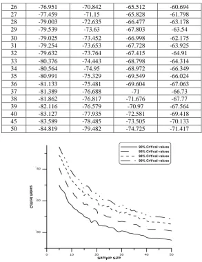
In this section a simulation for the null distribution critical points for δˆ will be made for sample sizes n=5(1)40, 45 and50 from the standard exponential distribution. Table-II gives the upper percentile of the statisticδˆ. Fig. (2) shows the relation between the critical values and the sample size.

Table II: Critical values of δˆ

n 90% 95% 98% 99%

5 -50.192 -39.886 -31.352 -26.02

6 -53.074 -43.752 -34.152 -29.611

7 -54.605 -46.201 -37.824 -32.537

8 -58.616 -49.8 -40.493 -35.458

9 -61.494 -52.483 -44.254 -39.611

10 -62.879 -54.027 -47.023 -41.644

11 -64.906 -56.765 -48.766 -44.04

12 -65.742 -58.541 -50.591 -45.291

13 -67.405 -60.365 -52.513 -46.797

14 -68.099 -60.16 -53.098 -49.005

15 -69.819 -62.708 -56.608 -52.38

16 -70.604 -62.593 -55.285 -50.611

17 -71.276 -64.857 -56.741 -51.73

18 -73.687 -66.149 -58.525 -54.204

19 -72.522 -65.468 -59.115 -55.195

20 -73.102 -66.429 -59.434 -55.236

21 -75.579 -70.166 -62.639 -56.546

22 -75.749 -69.969 -63.392 -59.021

23 -75.901 -69.505 -62.839 -59.473

24 -76.048 -70.449 -63.725 -59.554

25 -76.771 -70.775 -63.475 -59.634

0 0 1 2 3

.

5 1.5 2.5

λ

0 10 20 30 40

5 15 25 35

E

ff

ic

ie

nc

ISSN 2348 – 7968

26 -76.951 -70.842 -65.512 -60.694

27 -77.459 -71.15 -65.828 -61.798

28 -79.003 -72.635 -66.477 -63.178

29 -79.539 -73.63 -67.803 -63.54

30 -79.025 -73.452 -66.998 -62.175

31 -79.254 -73.653 -67.728 -63.925

32 -79.632 -73.764 -67.415 -64.91

33 -80.376 -74.443 -68.798 -64.314

34 -80.564 -74.95 -68.972 -66.349

35 -80.991 -75.329 -69.549 -66.024

36 -81.133 -75.481 -69.604 -67.063

37 -81.389 -76.688 -71 -66.73

38 -81.862 -76.817 -71.676 -67.77

39 -82.116 -76.579 -70.97 -67.564

40 -83.127 -77.935 -72.581 -69.418

45 -83.589 -78.485 -73.505 -70.133

50 -84.819 -79.482 -74.725 -71.417

Fig. (2) Relation between critical values and sample size for δˆ

7- Power of the test

In this section an estimation of the power for testing exponentiality versus EBURmgfR will be made using significance level 95% with suitable parameters values of θ at n=10,20 and 30, and for commonly used distributions in reliability such as LFR, Makeham, and Weibull alternatives. Table-III shows the power of the test.

Table-III: Power estimates

Distribution θ n

10 20 30

LFR

2 3 4

1 1 1

1 1 1

1 1 1

Makeham

2 3 4

0.998 1 1

1 1 1

1 1 1

Weibull

2 3 4

0.964 0.961 0.955

0.969 0.970 0.971

0.975 0.980 0.983 0 10 20 30 40 50

SampleSize

-80

-60

-40

C

r iti cal Va l

u

8-Example

The following data represent 39 liver cancer's patients taken from El-Minia Cancer Center of Ministry of Health of Egypt, in 1999. The ordered life times (in days) are:

The data are 10, 14, 14, 14, 14, 14, 15, 17, 18, 20, 20, 20, 20, 20, 23, 23, 24, 26, 30, 30, 31, 40, 49, 51, 52, 60, 61, 67, 71, 74, 75, 87, 96, 105, 107, 107, 107, 116, and 150.

It is found that the test statistic for the set of data by using equation (4.2) is δˆ= -1.57*10P

64

P

which is greater than the critical value of the Table-II, and then we accept HR1R which states that the set of data have EBURmgfR property at 95% percentile.

References

Ahmad, I. A. (2001). "Moments inequalities of aging families of distribution with hypothesis testing application". J. Statist. Plan. Inf., 92, 121-132.

Ahmad, I. A.& Sepehrifa, M. B. (2009)." On testing alternative classes of life distribution with guaranteed survival times". J. Comp.Statist. and Data Analysis, 857-864.

Elbatal, I. I. (2002). " The EBU and EWU classes of life distribution". J. Egypt. Statist. Soc., 18, 59-80.

Elbatal, I. I. (2007). " Some aging classes of life distributions at specific age". J. Int. math. Forum, 2, no.29, 1445-1456.

Kayid, M. & Diab, L. S. & Alzughaibi, A. (2010). " Testing NBU(2) class of life distribution based on goodness of fit approach". J. King Saud Univ.

Klar, B., & MÄuller, A.(2003)." Characterizations of classes of lifetime distributions generalizing the NBUE class". J.Appl.Prob.,40,20-32.

Lee, A. J. (1990). " U-statistic". MarcelDekker, New York, NY.