Copyright2000 by the Genetics Society of America
Quantitative Trait Loci: A Meta-analysis
Bruno Goffinet* and Sophie Gerber
†,1*INRA, Laboratoire de Biome´trie et d’Intelligence Artificielle, F-31326 Castanet-Tolosan Cedex, France and†INP/ENSAT, Laboratoire de Biotechnologie et d’Ame´lioration des Plantes, F-31326 Castanet-Tolosan Cedex, France
Manuscript received August 20, 1999 Accepted for publication January 24, 2000
ABSTRACT
This article presents a method to combine QTL results from different independent analyses. This method provides a modified Akaike criterion that can be used to decide how many QTL are actually represented by the QTL detected in different experiments. This criterion is computed to choose between models with one, two, three, etc., QTL. Simulations are carried out to investigate the quality of the model obtained with this method in various situations. It appears that the method allows the length of the confidence interval of QTL location to be consistently reduced when there are only very few “actual” QTL locations. An application of the method is given using data from the maize database available online at http://www.agron.missouri.edu/.
A
meta-analysis consists of combining data from dif- of qualitative developmental genes (KhavkinandCoe1997, 1998). ferent sources in a single study. This technique
is mainly used by researchers in medical, social, and Comparative analysis of QTL between species reveals
the existence of homologous QTL for plant height and
behavioral sciences (HedgesandOlkin1985). Its
appli-cation in genetics and evolution is illustrated in recent maturity within the Poaceae (sorghum, maize, rice,
wheat, and barley;Linet al. 1995). Similar observations
publications (Britten 1996; Allison and Heo 1998;
Van ZandtandMopper1998), and the usefulness of for traits involved in domestication suggest that few genes with a large effect have determined the pheno-these kinds of methods for pooling information when
raw data are not available is emphasized (Landerand types studied (Patersonet al. 1995). Comparing species
is also a means to find new QTL, increasing their
poten-Kruglyak1995;AllisonandHeo1998).
Since the first publication of a quantitative trait locus tial use for plant breeding, as in the tomato (Fulton
et al. 1997). Moreover, the existence of small common
(QTL) localization using molecular markers (Paterson
et al. 1988) a large number of species have been studied regions on linkage maps between taxa that diverged a long time ago may provide the opportunity to extend for numerous markers and traits. Some of the data
ob-tained are now available online, as in the maize database results obtained in one species (Patersonet al. 1996)
and permit the cross-utilization of resources that have (at http://www.agron.missouri.edu), where structured
been developed for a given species (Kowalski et al.
QTL data sets are continuously updated. Having data
1994). concerning different populations, it would be
interest-Several statistical methods to detect QTL have been ing to know whether QTL identified for a given trait in
developed (Jansen 1996). A QTL, once detected, is
one population correspond to those detected in other
described by its position on a linkage group, and possi-populations, or whether QTL locations identified in
bly a confidence interval around this position, an R2 or a one species correspond to QTL or other types of loci
lod score. When several crosses are available and studied detected in corresponding regions of other species. The
simultaneously for the same trait, a first statement is to QTL aspect of the database was created to encourage
consider that the QTL are common to both crosses but systematic description of QTL studies and to facilitate
that their alleles are different. Detecting QTL by interval
these kinds of comparisons (Byrneet al. 1995). Hence,
mapping consists then in testing at every point of the a recent revision of the QTL described in the database
chromosome the existence of a QTL with a potential suggests that QTL associations coincide with clusters
effect on each cross. This is the case when offspring of different males are considered in the same study in animal genetics with a model where the QTL effect is
Corresponding author: Bruno Goffinet, INRA, Laboratoire de
Biome´-different from one male to the other. This technique
trie et d’Intelligence Artificielle, Centre de Recherches de Toulouse,
F-31326 Castanet-Tolosan Cedex, France. is a way of increasing the QTL detection power when E-mail: [email protected]
the positions of the QTL are effectively the same 1Present address: INRA, Recherches Forestie`res, Laboratoire de
Ge´ne´-through the different crosses. However, when these
po-tique et Ame´lioration des Arbres Forestiers, BP 45, F-33611 Gazinet
Cedex, France. sitions are different, this method can mix them and
suggest “consensus” positions that do not actually corre- is the estimated QTL effect. We do not make use of this information in this article, except as a possible way, spond to any real position. The problem lies in testing
between one or several QTL in the same linkage group when combined with map density and the number of
observations, of estimating the variance of the QTL’s (Hyne and Kearsey 1995; Goffinet and Mangin
estimated position. Actually, the larger the QTL effect, 1998). Another statement is to estimate QTL
indepen-the smaller indepen-the var(xˆi).
dently in every cross and to test whether they are located
The n experiments are considered as independent. on the same place or not. When two crosses are
consid-This is clearly correct when the individuals measured ered, the similarity of the positions detected in the
in the different experiments are different. It is an ap-crosses can be tested by using confidence intervals for
proximation when these experiments represent differ-each position. When more than two QTL are involved,
ent traits measured on the same individuals or when the problem is more acute. The question to be answered
two or more QTL are detected for the same trait in an is not only whether there is a common position but also
experiment. We study in the simulation section the ef-to determine the number of different positions.
fect of considering independence between the experi-In this article we suggest an approach for choosing
ments when there are actually dependences between the best model to fit a set of data. Our aim was to
some experiments. Independence between experiment elaborate a meta-analysis of several QTL related to the
i and i⬘means independence between xˆiand xˆi⬘; that is,
same trait and mapped on the same linkage group in
basically the individuals used in the two experiments different independent studies. The question we wanted
are not the same, even supposing that the parent lines to address was the following: How many “real” QTL do
are the same. the QTL detected in the different studies represent—
one, two, three, or as many as the number detected
The set of xˆi, i⫽1, n is denoted Xˆ .
throughout the studies? Once this question is answered,
The different models: Let k ⫽ 1, . . . , n represent
the positions of the real QTL can be estimated. This
different models for the real position xiof the n QTL.
approach should help to gather data obtained from
In model k ⫽ 1, we consider that all the n QTL are
different populations and extract meaningful results for
located at a single position. In model k, we consider the species under investigation.
that there are k different positions for the n QTL, and model n corresponds to the case where the n QTL are located at n different positions.
METHODOLOGY
For each experiment i and model k we denote x˜i[k]the
The QTL experiment summary:Consider a set of n estimate of position x
i. We use the following estimates:
QTL experiments concerning the same linkage group.
k⫽1: x˜[1]
i ⫽ x⫽ 1⁄nRixˆi.
These different experiments may represent several
k ⫽ 2: [2]
1 and [2]2 are the maximum-likelihood
esti-crosses between different lines, or several sires, or
differ-mates of the possible values of xiin the two-population
ent traits, or different locations for the same trait, or
mixture model. To estimate these parameters, we con-different environmental conditions and experimental
sider all the possible distributions of the n QTL into designs.
two groups. For each distribution, we compute the
We consider that for each experiment i (i⫽ 1, . . . ,
maximum-likelihood estimator of the mean of each
n), the summary of the information is the estimated
group and choose the best distribution as the
distribu-position of the QTL xˆifor this experiment in this linkage
tion maximizing the likelihood.
group. We assume that the xˆiare normally distributed
around the true position xi of the QTL in experiment We have x˜[2]
i ⫽ [2]1 if |xˆi ⫺ 1[2] | ⬍ |xˆi ⫺ [2]2 | and i, with a variance var(xˆi)⫽ ␥E,i. As this variance can be x˜[2]
i ⫽ [2]2 otherwise.
generally estimated with a large number of observations,
k ⬍ n: The same rule as for k ⫽ 2 applies with [k] 1 ,
we assume that it is consistently estimated and therefore
[k]
2 , . . . ,[k]k the k possible values of the k-population
can be considered as known. Nevertheless, we
investi-mixture model. Notation [k] represents the number gate in the simulation section the effect of an imperfect
of QTL in this model. As for k ⫽2, we consider all
estimation of this parameter.
the possible distributions of the n QTL into k groups This Gaussian and unbiased approximation can be
con-and choose the distribution with the maximum likeli-sidered as correct for QTL with a large effect. In these
hood. cases, one can use the classical asymptotic Gaussian
dis-tribution of the maximum-likelihood estimation of the
We have x˜[k]
i ⫽ [k]j , where j is such that|xˆi ⫺ [k]j |is
parameters. For QTL with small effects,Manginet al.
minimum for j⫽ 1, . . . , k.
(1994) have shown that it is not perfectly correct. Never-theless, it is a simple and useful approximation and we
k⫽ n: x˜i[n]⫽xˆi.
consider it as correct for all the detected QTL.
crite-rion to choose from the different models k⫽1, . . . , Consider first, for example, the case n ⫽20, where
n. It is known (Titteringtonet al. 1985) that the Akaike more configurations are studied. The value of bias
de-criterion is not a correct way of comparing models in pends strongly upon the value of the number k0of
pa-the case of mixture models. We propose herein an adap- rameters in the actual model. Nevertheless, the main
tation of the Akaike criterion to deal with our models. aim of correcting the log-likelihood is to prevent the
Consider a model with k parameters⌰[k]⫽ [k]
1 ,[k]2 , choice of a model with more than k0parameters when
. . . , [k]
k and the n corresponding values of the QTL the number of parameters is actually k0. We observed
positions X⫽(xi)i⫽1,n. The log-likelihood of the observed that the difference between bias(X0, k0; k0) and bias (X0,
vector Xˆ is denoted L(⌰[k], X; Xˆ ). We denote k
0the actual k0; k0 ⫹ 1) depends little upon the values of X0. For
number of parameters,⌰[k]
0 the actual value of the pa- example, when the actual model has k0⫽2 parameters,
rameters, and X0the actual value of the n QTL positions. the difference between the bias when using a model
The maximum-likelihood estimates are denoted ⌰ˆ[k]
with 3 parameters and a model with 2 parameters is
and X˜[k] ⫽ (x˜[k]
i )i⫽1,n and the corresponding log-likeli- (see Table 1) 12.7⫺3.9⫽8.8 [configuration (config)
hood L(⌰ˆ[k], X˜[k]; Xˆ ).
2], or 10.6⫺2.0⫽8.6 (config 3), or 10.3⫺2.1⫽8.1
The aim of the Akaike criterion (Sakamoto et al. (config 4). This value tends to converge to a stable
1986) is to estimate the mean expected log-likelihood value as the difference between the parameters
i is
(MELL): increasing. We may therefore use the value 8.1 as a limit
value. These limit values are 13 for k0⫽1, 8.1 for k0⫽
MELL⫽E(⌰˜[k],X˜[k]
)(EX˜ *(L(⌰ˆ[k], X˜[k]; Xˆ *)).
2, 6.7 for k0⫽3, and 15.9 for k0⫽4. In this case, k0⫹
In the second expectation EXˆ *, the estimated values⌰ˆ[k], 1 is taken as n. We observed slightly different limit values
X˜[k]are fixed, and the expectation is taken for
indepen-when using unbalanced configurations (data not
dent possible values of observations Xˆ *, with the same shown).
probability distribution function as Xˆ . We propose, therefore, to use the following
expres-In regular situations, it is well known that L(⌰ˆ[k], X˜[k];
sions of AIC*(k) to choose from the models k⫽ 1, 2,
Xˆ ) ⫺ k, where k is the number of free parameters of 3, 4, n⫽20:
the model, is an asymptotically unbiased estimator of
MELL. Therefore, it is recommended to choose a model AIC*(1)⫽ ⫺2⫻ (L(⌰ˆ[1], X˜[1]; Xˆ ) ⫺1)
minimizing the Akaike information criterion, AIC ⫽
AIC*(2)⫽ ⫺2⫻ (L(⌰ˆ[2], X˜[2]; Xˆ ) ⫺1⫺13)
⫺2⫻L(⌰ˆ[k], X˜[k]; Xˆ ) ⫹2⫻
k.
In our cases of mixtures models, L(⌰ˆ[k], X˜[k]; Xˆ )⫺ k
AIC*(3)⫽ ⫺2⫻ (L(⌰ˆ[3], X˜[3]; Xˆ ) ⫺1⫺13⫺ 8.1)
is not an unbiased estimator of MELL, except for k⫽
AIC*(4)⫽ ⫺2⫻ (L(⌰ˆ[4], X˜[4]; Xˆ ) ⫺1⫺13
1 and k ⫽ n. We propose to estimate numerically
bias (X0, k0; k)⫽MELL⫺E(L(⌰ˆ[k], X˜[k]; Xˆ )) in different ⫺8.1 ⫺6.7)
situations. Table 1 shows the values of this bias for
differ-AIC*(20) ⫽ ⫺2⫻ (L(⌰ˆ[n], X˜[n]; Xˆ )⫺ 1⫺ 13⫺8.1
ent values of n and k, and different values of k0and X0
of the actual model, that is, when using a model with ⫺6.7 ⫺15.9)
k parameters when there are actually k0parameters and
the actual parameter values are X0. The different con- It appears that these coefficients are approximately
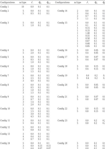
con-figurations l, l⫽ 1, 10 are described in Table 2. The stant or a linear function of n when n changes. We can
therefore propose the following expressions for AIC*(k)
computations are based onE,i⫽
√
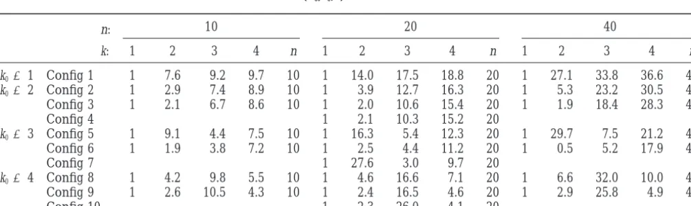
␥E,i⫽10 cM.TABLE 1
Value of bias(X0,k0;k) in different situations
10 20 40
n:
k: 1 2 3 4 n 1 2 3 4 n 1 2 3 4 n
k0⫽1 Config 1 1 7.6 9.2 9.7 10 1 14.0 17.5 18.8 20 1 27.1 33.8 36.6 40
k0⫽2 Config 2 1 2.9 7.4 8.9 10 1 3.9 12.7 16.3 20 1 5.3 23.2 30.5 40
Config 3 1 2.1 6.7 8.6 10 1 2.0 10.6 15.4 20 1 1.9 18.4 28.3 40
Config 4 1 2.1 10.3 15.2 20
k0⫽3 Config 5 1 9.1 4.4 7.5 10 1 16.3 5.4 12.3 20 1 29.7 7.5 21.2 40
Config 6 1 1.9 3.8 7.2 10 1 2.5 4.4 11.2 20 1 0.5 5.2 17.9 40
Config 7 1 27.6 3.0 9.7 20
k0⫽4 Config 8 1 4.2 9.8 5.5 10 1 4.6 16.6 7.1 20 1 6.6 32.0 10.0 40
Config 9 1 2.6 10.5 4.3 10 1 2.4 16.5 4.6 20 1 2.9 25.8 4.9 40
TABLE 2
Description of the configurations forn⫽10 experiments
Configurations m/type i E,i E,i;0 Configurations m/type i E,i E,i;0
Config 1 10 0.0 0.1 0.1
Config 2 5 0.0 0.1 0.1 Config 14 2 0.0 0.1 0.1
5 0.5 0.1 0.1 3 0.4 0.1 0.1
2 0.7 0.1 0.1
3 1.1 0.1 0.1
Config 3 5 0.0 0.1 0.1 Config 15 1 0.0 0.1 0.1
5 1.0 0.1 0.1 1 0.1 0.1 0.1
1 0.15 0.1 0.1
1 0.33 0.1 0.1
1 1.48 0.1 0.1
1 0.55 0.1 0.1
1 0.58 0.1 0.1
1 0.67 0.1 0.1
1 0.68 0.1 0.1
1 0.85 0.1 0.1
Config 4 5 0.0 0.1 0.1 Config 16 5 0.0 0.05 0.05
5 2.0 0.1 0.1 5 0.4 0.05 0.05
Config 5 4 0.0 0.1 0.1 Config 17 5 0.0 0.07 0.07
3 0.5 0.1 0.1 5 0.4 0.07 0.07
3 1.0 0.1 0.1
Config 6 3 0.0 0.1 0.1 Config 18 5 0.0 0.15 0.15
4 1.0 0.1 0.1 5 0.4 0.15 0.15
3 1.5 0.1 0.1
Config 7 3 0.0 0.1 0.1 Config 19 5 0.0 0.2 0.2
4 2.5 0.1 0.1 5 0.4 0.2 0.2
3 4.0 0.1 0.1
Config 8 3 0.0 0.1 0.1 Config 20 5 0.0 0.05 0.05
2 0.5 0.1 0.1 5 0.8 0.05 0.05
2 1.0 0.1 0.1
3 1.5 0.1 0.1
Config 9 2 0.0 0.1 0.1 Config 21 5 0.0 0.07 0.07
3 0.7 0.1 0.1 5 0.8 0.07 0.07
3 1.4 0.1 0.1
2 2.0 0.1 0.1
Config 10 2 0.0 0.1 0.1 Config 22 5 0.0 0.15 0.15
3 1.5 0.1 0.1 5 0.8 0.15 0.15
3 3.0 0.1 0.1
2 4.5 0.1 0.1
Config 11 5 0.0 0.1 0.1 Config 23 5 0.0 0.2 0.2
5 0.4 0.1 0.1 5 0.8 0.2 0.2
Config 12 5 0.0 0.1 0.1
5 0.8 0.1 0.1
Config 13 3 0.0 0.1 0.1
4 0.4 0.1 0.1
3 0.7 0.1 0.1
Config 24 5 0.0 0.1 0.1 Config 28 5 0.0 0.1 0.1
3 0.0 0.15 0.15 3 0.0 0.1 0.15
2 0.0 0.07 0.07 2 0.0 0.1 0.07
TABLE 2
(Continued)
Configurations m/type i E,i E,i;0 Configurations m/type i E,i E,i;0
Config 25 2 0.0 0.1 0.1 Config 29 2 0.0 0.1 0.1
3 0.0 0.07 0.07 3 0.0 0.1 0.07
3 0.4 0.15 0.15 3 0.4 0.1 0.15
2 0.4 0.1 0.1 2 0.4 0.1 0.1
Config 26 3 0.0 0.1 0.1 Config 30 3 0.0 0.1 0.1
2 0.0 0.07 0.07 2 0.0 0.1 0.07
3 0.8 0.15 0.15 3 0.8 0.1 0.15
2 0.8 0.1 0.1 2 0.8 0.1 0.1
Config 27 2 0.0 0.1 0.1 Config 31 2 0.0 0.1 0.1
1 0.0 0.07 0.07 1 0.0 0.1 0.07
1 0.5 0.1 0.1 1 0.5 0.1 0.1
1 0.5 0.07 0.07 1 0.5 0.1 0.07
1 1.0 0.15 0.15 1 1.0 0.1 0.15
1 1.0 0.1 0.1 1 1.0 0.1 0.1
2 1.5 0.15 0.15 2 1.5 0.1 0.15
1 1.5 0.1 0.1 1 1.5 0.1 0.1
Config 32 5 0.0 0.1 0.1 Correlation
3 0.0 0.1 0.15 ⫽0.8
2 0.0 0.1 0.07 between 1,2; 3,4; etc.
Config 33 2 0.0 0.1 0.1 Correlation
3 0.0 0.1 0.07 ⫽0.8
3 0.4 0.1 0.15 between 1,2; 3,4; etc.
2 0.4 0.1 0.1
Config 34 3 0.0 0.1 0.1 Correlation
2 0.0 0.1 0.07 ⫽0.8
3 0.8 0.1 0.15 between 1,2; 3,4; etc.
2 0.8 0.1 0.1
Config 35 2 0.0 0.1 0.1 Correlation
1 0.0 0.1 0.07 ⫽0.8
1 0.5 0.1 0.1 between 1,2; 3,4; etc.
1 0.5 0.1 0.07
1 1.0 0.1 0.15
1 1.0 0.1 0.1
2 1.5 0.1 0.15
1 1.5 0.1 0.1
For n⫽20, each configuration is doubled (⫻4 for n⫽40). m/type is the number of experiments of the type described in the line that is with an actual expectationiand actual standard deviationE,i;0;E,iis the
standard deviation used in the simulations for this type.
that can be used for any value of n such that 10ⱕnⱕ efficient when n becomes ⬎40 or for chromosome
40: length⬎2 M.
The expressions for AIC*(k) were obtained using a
AIC*(1)⫽ ⫺2⫻ (L(⌰ˆ[1], X˜[1]; Xˆ )⫺ 1)
particular situation for the E,i and independence
be-AIC*(2)⫽ ⫺2⫻ (L(⌰ˆ[2], X˜[2]; Xˆ )⫺ 0.7⫻n) tween the xˆ
i. Nevertheless, we propose to use these
ex-pressions in general situations including different and
AIC*(3)⫽ ⫺2⫻ (L(⌰ˆ[3], X˜[3]; Xˆ )⫺ 1.11⫻n)
variable values for theE,iand nonindependence. Their
AIC*(4)⫽ ⫺2⫻ (L(⌰ˆ[4], X˜[4]; Xˆ )⫺ 1.44⫻n)
efficiencies in these situations are investigated by simula-tions in the following section.
AIC*(n) ⫽ ⫺2⫻ (L(⌰ˆ[n], X˜[n]; Xˆ )⫺2.27⫻ n).
Note that we do not propose expressions for k⫽ 5,
. . . , n ⫺ 1. The reason for that is the inefficiency of
COMPARISON OF MODEL SELECTION STRATEGIES
the use of the corresponding models when 10ⱕ n ⱕ
Alternative strategies and comparison indicators:We
40 and the length of chromosome is shorter than 2 M.
obtained with the two alternative strategies of choosing val in a QTL experiment, one needs to use four times
a model: the initial number of observations. The conventional
strategy S1 becomes equal or better when there are
strategy S1. x˜i(S1)⫽xˆi. This is the “conventional” strategy, many actual positions (config 15) or when the actual
which retains the estimated position.
QTL positions are narrow in regard to variance
(con-strategy S2. Choose the model l2 giving the minimum fig 4, 18, and 19). Nevertheless, the greatest loss is
value of the AIC*(l2) criterion. The corresponding ⵑ
20% for the confidence intervals. Except for config estimate of xiis x˜i(S2)⫽ x˜[l2]i .
13, the conclusions are the same for the three compar-ison indicators.
For each of these h⫽1, 2 strategies, we compute two
Step 2. Configurations 24–27: When comparing config kinds of indicators:
24 with config 1, and config 26 with config 12, it
The mean squared error of prediction RSh ⫽ 1⁄
n Rni⫽1
appears that the variability among the E,idoes not
E(xi⫺x˜i(Sh))2.
change the behavior of the strategies for all the crite-The length of the confidence interval at 95 and 90%
ria. Nevertheless, the comparisons between config 25 for the position of the QTL. To obtain this length,
with config 11 and config 27 with config 8 show that
we compute the quantities|xi⫺x˜i(Sh)|and calculate
the gain in using S2is less when there is a variability
the quantiles q(0.95) and q(0.90) of its empirical
dis-among the variances when using the 0.95% tribution over all the QTL. The smaller this
confi-dence interval criterion. The difference between
con-dence interval, the better the location estimator x˜i(Sh).
fig 25 and 11 is more important than the difference
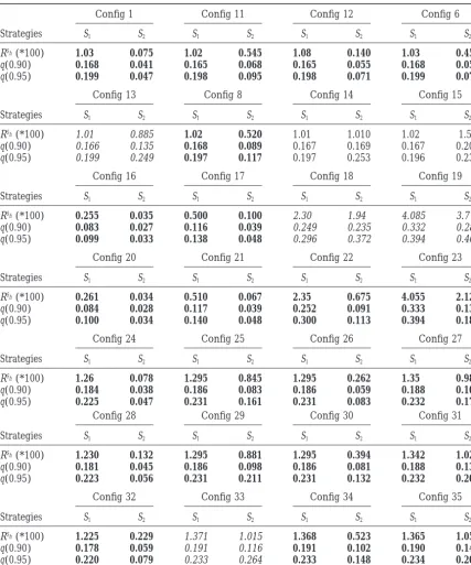
Simulation results:We compare different configura- between config 24 and 1 because it is possible to
tions concerning k0 and X0 in four steps. In the first detect two populations whose means differ by 0.4 with
step, we consider the standard deviation E,i⫽
√
␥E,i as E,i⫽ 0.1, but it becomes more difficult whenE,i⫽constant among i⫽1, n and known; that is, the actual 0.15.
standard deviation E,i;0 used in the simulations is the Step 3. Configurations 28–31: As previously, the
compar-same as the standard deviationE,iused in the model. isons between config 24 and 28 and between config
In the second step, the standard deviations are known 26 and 30 show some decrease in the gain when using
but different from one observation i to another. In the S2, but not a very substantial one. The gain in using S2
third step, the standard deviations are different and for the 95% confidence interval continues to decrease
unknown; that is, the standard deviation E,i;0 used in when comparing config 25 with 29 and config 27 with
the simulations is different from the standard deviation 31.
of the model. In the fourth step, we investigate the Step 4. Configurations 32–35: Globally the comparisons
effect of nonindependence between the experiments between config 28 and 32, config 29 and 33, config
by adding into the simulation model a correlation ⫽ 30 and 34, and config 31 and 35 show a small decrease
0.8 between xˆi and xˆi⬘for i⫽1 and i⬘ ⫽2, i⫽ 3, and in the gain when using S2for the different indicators.
i⬘ ⫽ 4 and so on. This choice is arbitrary. In all these
cases, the number of observations is n⫽20, the xˆivalues Nevertheless, the use of S2in all these configurations
are simulated as normally distributed N(xi, ␥E,i;0), and continues to be advantageous (config 35) or very
advan-we perform 500 simulations. The configurations are tageous (config 32 and 34) for all the indicators. The
described in Table 2 and the results in Table 3. The conclusions are less clear for config 33, as it depends
reason for the choice of n⫽20 is that it is a common on the indicator.
number of experiments that are presently found in the We do not give the loss in gain for all types of
configu-literature. The choice of the configurations is linked to rations through the three last steps. For example, the
the length of maize chromosomes (between 1 and 2 series config 20, 26, 30, and 34 have the same behavior
M). The configurations try to cover the range of possible as the same kind of series beginning with config 6.
repartitions of QTL positions. It does not try to be a Discussion:The results show that if there are actually
“sample” of the reality as we do not know what the reality one, two, three, or four different locations for the QTL
is. In Table 3, we give the value of the mean squared studied, strategy S
2proposed in this article is able to give
error of prediction RSh, and the mean length of the 90
a better estimation of the xi than the use of estimated
and 95% confidence interval of the QTL position, for
positions xˆi. The different comparison indicators try to
both strategies S1and S2. measure the quality of this estimation. They give
consis-tent results. Our method combines different QTL loca-Step 1. Configurations 1–23: It appears that the gain
tion estimates xˆi, as is usually done in meta-analysis
stud-obtained with strategy S2is substantial in several
situa-ies even if they manipulate other types of data (e.g., tions for the different comparison indicators. For
ex-Britten1996;AllisonandHeo1998;Van Zandtand ample, the length of the 95% confidence interval is
Mopper1998;Vøllestad et al. 1999). However, these
divided by 4.5 when using S2 when there is actually
studies deal with what would correspond to only one only one QTL position. In several situations, this
TABLE 3
Mean squared error of predictionRSh, length of the confidence interval at 90%q(0.90) [respectively,
95%q(0.95)] computed with 500 simulations in different configurations for both strategies
Config 1 Config 11 Config 12 Config 6
Strategies S1 S2 S1 S2 S1 S2 S1 S2
RSh(*100) 1.03 0.075 1.02 0.545 1.08 0.140 1.03 0.455
q(0.90) 0.168 0.041 0.165 0.068 0.165 0.055 0.168 0.056
q(0.95) 0.199 0.047 0.198 0.095 0.198 0.071 0.199 0.071
Config 13 Config 8 Config 14 Config 15
Strategies S1 S2 S1 S2 S1 S2 S1 S2
RSh(*100) 1.01 0.885 1.02 0.520 1.01 1.010 1.02 1.50
q(0.90) 0.166 0.135 0.168 0.089 0.167 0.169 0.167 0.203
q(0.95) 0.199 0.249 0.197 0.117 0.197 0.253 0.196 0.238
Config 16 Config 17 Config 18 Config 19
Strategies S1 S2 S1 S2 S1 S2 S1 S2
RSh(*100) 0.255 0.035 0.500 0.100 2.30 1.94 4.085 3.775
q(0.90) 0.083 0.027 0.116 0.039 0.249 0.235 0.332 0.281
q(0.95) 0.099 0.033 0.138 0.048 0.296 0.372 0.394 0.400
Config 20 Config 21 Config 22 Config 23
Strategies S1 S2 S1 S2 S1 S2 S1 S2
RSh(*100) 0.261 0.034 0.510 0.067 2.35 0.675 4.055 2.120
q(0.90) 0.084 0.028 0.117 0.039 0.252 0.091 0.333 0.136
q(0.95) 0.100 0.034 0.140 0.048 0.300 0.113 0.394 0.185
Config 24 Config 25 Config 26 Config 27
Strategies S1 S2 S1 S2 S1 S2 S1 S2
RSh(*100) 1.26 0.078 1.295 0.845 1.295 0.262 1.35 0.980
q(0.90) 0.184 0.038 0.186 0.083 0.186 0.059 0.188 0.109
q(0.95) 0.225 0.047 0.231 0.161 0.231 0.083 0.232 0.178
Config 28 Config 29 Config 30 Config 31
Strategies S1 S2 S1 S2 S1 S2 S1 S2
RSh(*100) 1.230 0.132 1.295 0.881 1.295 0.394 1.342 1.025
q(0.90) 0.181 0.045 0.186 0.098 0.186 0.081 0.188 0.133
q(0.95) 0.223 0.056 0.231 0.211 0.231 0.132 0.232 0.203
Config 32 Config 33 Config 34 Config 35
Strategies S1 S2 S1 S2 S1 S2 S1 S2
RSh(*100) 1.225 0.229 1.371 1.015 1.368 0.523 1.365 1.056
q(0.90) 0.178 0.059 0.191 0.116 0.191 0.102 0.190 0.144
q(0.95) 0.220 0.079 0.233 0.264 0.233 0.148 0.234 0.209
The values are indicated in boldface when S2is better than S1for all the indicators and in italic when no
strategy is better for all the indicators. See Table 2 for a description of configurations.
The theory is developed for independent experi- A particular situation is the case where two different
QTL are detected on the same chromosome for the ments and known variance. We apply this theory for
nonindependent observations in the simulation section same trait and in the same experiment. In this case,
considering the two QTL as independent will not take and consider the effect of imperfect knowledge of the
variance. The quality of the results in these cases shows the previous information into account.
Imagine a situation where we have all the markers that the method is robust and that there is no need for
a specific theory to take nonindependence and estima- and phenotypic information for the different
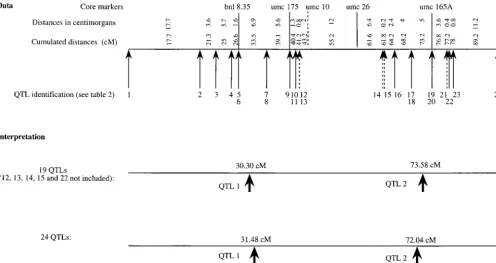
Figure1.—QTL related to yield on linkage group 3 of the maize genome.
be possible to perform a global linkage analysis and to we discard them from the analysis and use only the
other 19 QTL.
look for common QTL in each position as inHaleyet
al. (1994) orRebaiandGoffinet(1993). The question Our linkage data span from bin 3.4 to bin 3.6 ac-cording to the nomenclature of the maize database. of distinguishing between one, two, three or more QTL
becomes a different problem in this case. As shown, for Looking through the different studies in which the
data were collected, we were able to estimate confidence
example, inGoffinetandMangin(1998), the
distinc-tion between these different hypotheses is not easy. intervals for the majority of QTL positions. If we
con-sider these positions to be normally distributed and a
The expressions for AIC*(k) are given for k ⫽ 1, 2,
3, 4, n. It would be interesting to obtain this expression confidence interval C(90) of 90%, the standard
devia-tions E,i of the different QTL can be estimated as
for k ⬎ 4, but as noted previously, it would only be
useful for values of n ⬎ 40 and for a chromosome C(90)⫽2⫻1.645⫻ E,icM. These values are given in
Table 4. For those QTL where no confidence interval
whose length is⬎2 M. However, according to the dense
linkage maps existing nowadays for many different spe- could be evaluated, the value ofE,iwas taken as 6, 10,
or 15 cM, corresponding to confidence intervals of 20, cies, mean chromosome lengths never exceed this value.
33, or 50 cM, the second value equaling the mean of our estimated confidence intervals. The QTL number
AN APPLICATION USING THE MAIZE 1 is quite far from the others. This QTL must have a
GENOME DATABASE
large variance: its position is likely to be inaccurately
Using the maize database (at http://www.agron. estimated, since it is located in an interval of 42.6 cM
missouri.edu), we collected the data concerning QTL without any marker and 16 cM apart from the nearest
related to yield and located on linkage group 3. We marker (VeldboomandLee1996). For these reasons,
looked through the original publications and were able we attributed a E,i of 20 cM to this QTL for further
to construct a “consensus” map, where all the QTL could analysis.
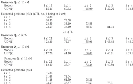
be localized. This map was based on core markers that We first tested our model with 19 QTL, with aEof
were present in the different publications. The distances 10 cM; then we included the 5 QTL localized relative
between two markers could differ between publications to marker umc10 in the data, that is, 24 QTL with the
but were quite similar: we took the average values for different values ofE,i. The results are given in Table 5
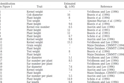
our map. A total of 24 QTL could be detected; their and are discussed in the next section.
position is given in Figure 1, and their description is in Discussion:In Table 5, the underlined number is the
Table 4. Five of them were mapped relative to marker best value of the criterion. In all cases, the model with
umc10 (QTL numbers 12, 13, 14, 15, and 21), whose two positions is favored by the criteria, whatever the
value ofEand the number of QTL considered.
TABLE 4
QTL related to yield on linkage group 3 of the maize genome
Identification Estimated
in Figure 1 Trait E,i(cM) Reference
1 Kernel weight a VeldboomandLee(1996)
2 Cob diameter 16 Beaviset al. (1994)
3 Plant height 8 Beaviset al. (1994)
4 Test weight a Ajmone-Marsanet al. (1995)
5 Plant height 9.6 Beaviset al. (1994)
6 Kernel row number 6.5 AustinandLee(1996)
7 Plant height 12 Beaviset al. (1991)
8 Plant height 12 Beaviset al. (1991)
9 Plant height 6.7 Scho¨ net al. (1993)
10 Kernel weight 9.8 AustinandLee(1996)
11 Kernel weight 15.3 VeldboomandLee(1994)
12 Grain weight a Maize Database, CIMMYT (1994)b
13 Plant height a Maize Database, CIMMYT (1994)b
14 Test weight 8 Beaviset al. (1994)
15 Plant height a Maize Database, CIMMYT (1994)b
16 Ear diameter 5.1 VeldboomandLee(1994)
17 Ear number per plant 8.5 VeldboomandLee(1994)
18 Ear number per plant a VeldboomandLee(1996)
19 Ear diameter 7.6 AustinandLee(1996)
20 Kernel weight 7.6 AustinandLee(1996)
21 Plant height a Maize Database, CIMMYT (1994)b
22 Ear number per plant 5.5 AustinandLee(1996)
23 Plant height 14.9 Scho¨ net al. (1994)
24 Ear length 6.8 VeldboomandLee(1994)
aNo information available in the reference.
bhttp://www.agron.missouri.edu:80/cgi_bin/sybgw_mdb/mdb3/reference/67081.
The 19 QTL are well represented by two real QTL a given QTL is very small; there are many possible genes,
located on positions 30.30 (QTL 1) and 73.58 (QTL and the candidate can be chosen in two different ways.
2; see large arrows in Figure 1). QTL 1–11 would be First, the candidate gene can be chosen on an a priori
representative of a first QTL at 30.30 cM, QTL 16–24 belief that, due to its function, the gene is associated
would be a second one at 73.58 cM (Figure 1). The trait with the trait of interest. Second, the gene can be
sus-affected by QTL 1 is mainly plant height whereas QTL pected to be the candidate because it is located in the
2 mainly affects ear traits (Table 4). area of the QTL: this is a positional comparative
candidate-When the QTL located relative to locus umc10 are gene analysis (RotschildandSoller1997). Unless the
included in the analysis, the results are not much af- QTL position confidence interval is very narrow, the initial
fected [Table 5 (24 QTL) and Figure 1]. The estimation candidate gene can be incorrect. To increase the power
of the positions for the models with two QTL are close of detection, the confidence interval must be narrowed,
to those estimated with 19 QTL. or the results from several genome-wide surveys must
be combined (Keightleyet al. 1998), which is precisely
what we suggest in this study. Gathering QTL data
to-CONCLUSION gether should be a good way to obtain a better
estima-tion of a QTL posiestima-tion and thus to specify a colocaestima-tion As the number of studies concerning QTL detection
with a candidate gene. Moreover, the reduction of the increases, articles dealing with the use of results from
confidence interval associated with QTL location is an several studies concentrating on different species
important goal (see, for instance, Kearsey and
Far-(Kearsey and Farquhar 1998) or on a single one
quhar1998), so the reduction provided by the method (Khavkin and Coe 1997, 1998) are now available. A
presented in this article is therefore of advantage. major step toward a more accurate identification of a
In the maize genome, functional clusters were found QTL consists of finding the proper candidate gene.
associating QTL and genes for growth, development, A candidate gene for a given trait is a sequence of a
and stress response. The genomic location of the QTL gene of a known biological function involved with the
used in our example (chromosome 3, bins 4–6) con-development or physiology of the trait. However, the
TABLE 5
Application of the models to the maize data
19 QTL (QTL nos. 12, 13, 14, 15, and 22 not included)
UnknownE,i⫽10 cM
Models k⫽19 k⫽1 k⫽2 k⫽3 k⫽4
AIC*(k) ⫺15.41 60.33 ⫺45.94a ⫺37.26 ⫺32.35
Estimated positions (cM) (QTL no. 1 being at 0 cM)
k⫽1 54.86
k⫽2 30.30 73.58
k⫽3 23.59 38.19 73.58
k⫽4 23.59 38.19 68.40 81.34
24 QTL UnknownE,i⫽6 cM
Models k⫽24 k⫽1 k⫽2 k⫽3 k⫽4
AIC*(k) ⫺23.39 72.97 ⫺55.96 ⫺48.45 ⫺45.09
UnknownE,i⫽10 cM
Models k⫽24 k⫽1 k⫽2 k⫽3 k⫽4
AIC*(k) ⫺17.26 44.10 ⫺56.08 ⫺45.91 ⫺39.53
UnknownE,i⫽15 cM
Models k⫽24 k⫽1 k⫽2 k⫽3 k⫽4
AIC*(k) ⫺12.40 37.94 ⫺53.34 ⫺42.50 ⫺34.87
Estimated positions (cM)
k⫽1 55.09
k⫽2 31.48 72.04
k⫽3 31.48 64.59 78.36
k⫽4 23.59 38.87 64.59 78.3
aUnderlined, best value of the criterion.
genes for reduced or distorted growth of shoot, leaf, vides a framework for the comparative analysis of
com-plex phenotypes (Paterson et al. 1995). Using
meta-male and femeta-male inflorescence, loci for reduced plant
vigor, and loci for a transcription binding factor (Khav- analysis to extract meaningful results for a particular
species may in this way have a greater impact.
kin andCoe 1997). Moreover, according to these
au-thors, chromosomes 1 and 3 seem to carry 40% of all developmental genes. Thanks to the associated skills of
LITERATURE CITED
physiologists and geneticists, as a growing number of
genes are mapped and as their function is increasingly Ajmone-Marsan, P., G. Monfredini, W. F. Ludwig, A. E.
Mel-chinger, P. Franceschiniet al., 1995 In an elite cross of maize
well elucidated, the number of potential candidate
a major quantitative trait locus controls one-fourth of the genetic
genes is increasing. Tools are needed to determine the variation for grain yield. Theor. Appl. Genet. 90: 415–424.
relevant candidate, and specifying a colocation is one Allison, D. B.,and M. Heo, 1998 Meta-analysis of linkage data
under worst-case conditions: a demonstration using the human
of them.
OB region. Genetics 148: 859–865.
The correspondence of QTL across genomes of dif- Austin, D. F.,andM. Lee,1996 Comparative mapping in F2:3 and
ferent species is illustrated by several studies, for in- F6:7 generations of quantitative trait loci for grain yield and yield
components in maize. Theor. Appl. Genet. 92: 817–826.
stance between different Brassica species and
Arabi-Beavis, W. D., D. Grant, M. Albertsen and R. Fincher, 1991
dopsis, where the potential of integrating QTL analysis Quantitative trait loci for plant height in four maize populations
with comparative studies and candidate loci suggested and their associations with qualitative genetic loci. Theor. Appl.
Genet. 83: 141–145.
by the synteny Brassica/Arabidopsis is highlighted for
Beavis, W. D., O. S. Smith, D. GrantandR. Fincher,1994
Identi-flowering traits (Bohuonet al. 1998). Comparative map- fication of quantitative trait loci using a small sample of topcrossed
ping yields a more comprehensive list of QTL than can and F4 progeny from maize. Crop Sci. 34: 882–896.
Bohuon, E. J. R., L. D. Ramsay, J. A. Craft, A. E. Arthur, D. F.
be obtained from any individual population (Linet al.
Marshallet al., 1998 The association of flowering time
quanti-1995), so a meta-analysis approach can be performed tative trait loci with duplicated regions and candidate loci in
within a species, and the result obtained can be tested Brassica oleracea. Genetics 150: 393–401.
Britten, H. B., 1996 Meta-analysis of the association between
on another species. The existence of model species on
multilocus heterozygosity and fitness. Evolution 50: 2158–2164.
which studies are concentrated facilitates meta-analysis. Byrne, P. F., M. B. Berlyn, E. H. Coe, G. L. Davis, M. L. Polacco
et al., 1995 Reporting and accessing QTL information in USDA’s
pro-Maize Genome Database. J. Quant. Trait Loci (at http://probe. Lincolnet al., 1988 Resolution of quantitative traits into men-delian factors by using a complete linkage map of restriction nalusda.gov:8000/otherdocs/jqtl/index.html).
Fulton, T. M., T. Beckbunn, D. Emmatty, Y. Eshed, J. Lopezet fragment length polymorphisms. Nature 335: 721–726.
Paterson, A. H., Y. R. Lin, Z. Li, K. F. Schertz, J. F. Doebleyet al.,
al., 1997 QTL analysis of an advanced backcross of Lycopersicon
peruvianum to the cultivated tomato and comparisons with QTLs 1995 Convergent domestication of cereal crops by independent mutations at corresponding genetic loci. Science 269: 1714–1718. found in other wild species. Theor. Appl. Genet. 95: 881–894.
Goffinet, B.,andB. Mangin,1998 Comparing methods to detect Paterson, A. H., T. H. Lan, K. P. Reischmann, C. Chang, Y. R. Lin
et al., 1996 Toward a unified genetic map of higher plants, more than one QTL on a chromosome. Theor. Appl. Genet. 96:
transcending the monocot-dicot divergence. Nat. Genet. 14: 380– 628–633.
382.
Haley, C. S., S. A. KnottandJ. M. Elsen,1994 Mapping
quantita-Rebai, A.,andB. Goffinet,1993 Power of tests for QTL detection
tive trait loci in crosses between outbred lines using least squares.
using replicated progenies derived from a diallel cross. Theor. Genetics 136: 1195–1207.
Appl. Genet. 86: 1014–1022.
Hedges, L. V.,andI. Olkin,1985 Statistical Methods for Meta-Analysis.
Rotschild, M. F., andM. Soller,1997 Candidate gene analysis
Academic Press, Orlando, FL.
to detect genes controlling traits of economic importance in
Hyne, V.,andM. J. Kearsey,1995 QTL analysis: further uses of
domestic livestock. Probe 8: 13–20. ‘marker regression’. Theor. Appl. Genet. 91: 471–476.
Sakamoto, Y., M. IshiguroandG. Kitagawa,1986 Akaike
Informa-Jansen, R. C.,1996 Complex plant traits: time for polygenic analysis.
tion Criterion Statistics. KTK Scientific Publishers, Tokyo. Trends Plant Sci. 1: 89–94.
Scho¨ n, C. C., M. Lee, A. E. Melchinger, W. D. GuthrieandW. L.
Kearsey, M. J.,andA. G. L. Farquhar,1998 QTL analysis in plants:
Woodman,1993 Mapping and characterization of quantitative
where are we now? Heredity 80: 137–142.
trait loci affecting resistance against second-generation European
Keightley, P. D., K. H. Morris, A. Ishikawa, V. M. Falconerand
corn borer in maize with the aid of RFLPs. Heredity 70: 648–659.
F. Oliver,1998 Test of candidate gene-quantitative trait locus
Scho¨ n, C. C., A. E. Melchinger, J. Boppenmaier, E.
Brunklaus-association applied to fatness in mice. Heredity 81: 630–637.
Junget al., 1994 RFLP mapping in maize: quantitative trait loci
Khavkin, E.,andE. H. Coe,1997 Mapped genomic locations for
affecting testcross performances of elite european flint lines. developmental functions and QTLs reflect concerted groups in
Crop Sci. 34: 378–389. maize (Zea mays L.). Theor. Appl. Genet. 95: 343–352.
Titterington, D. M., A. F. M. SmithandU. E. Makov,1985
Statisti-Khavkin, E.,andE. H. Coe,1998 The major quantitative trait loci
cal Analysis of Finite Mixture Distributions. John Wiley & Sons, New for plant stature, development and yield are general
manifesta-York. tions of developmental gene clusters. Maize Newslett. 72: 60–66.
Van Zandt, P.,andS. Mopper,1998 A meta-analysis of adaptive
Kowalski, S. P., T. H. Lan, K. A. FeldmannandA. H. Paterson,
deme formation in phytophagous insect populations. Am. Nat. 1994 Comparative mapping of Arabidopsis thaliana and Brassica 152:595–604.
oleracea chromosomes reveals islands of conserved organization. Veldboom, L. R., andM. Lee,1994 Molecular-marker-facilitated Genetics 138: 499–510. studies of morphological traits in maize. II. Determination of
Lander, E.,andL. Kruglyak,1995 Genetic dissection of complex QTLs for grain yield and yield components. Theor. Appl. Genet.
traits: guidelines for interpreting and reporting results. Nat. 89:451–458.
Genet. 11: 241–247. Veldboom, L. R.,andM. Lee,1996 Genetic mapping of quantitative
Lin, Y. R., K. F. SchertzandA. H. Paterson,1995 Comparative trait loci in maize in stress and nonstress environments. I. Grain
analysis of QTLs affecting plant height and maturity across the yield and yield components. Crop Sci. 36: 1310–1319.
poaceae, in reference to an interspecific sorghum population. Vøllestad, L. A., K. HindarandA. P. Møller,1999 A meta-analysis Genetics 141: 391–411. of fluctuating asymmetry in relation to heterozygosity. Heredity
Mangin, B., B. GoffinetandA. Rebai,1994 Constructing confi- 83:206–218.
dence intervals for QTL location. Genetics 138: 1301–1308.