JONES, MARTHA LOUISE. A Retrospective Method for Inference on Haplotype Main Effects and Haplotype-environment Interactions Using Clustered Haplotypes. (Under the direction of Dr. Jung-Ying Tzeng.)
Many regression-based methods exist for conducting haplotype association analysis in case-control studies. Such methods generally are based on either a prospective frame-work (modeling the probability of disease conditional on haplotypes and covariates) or a retrospective framework (modeling the probability of haplotypes and covariates con-ditional on disease). For haplotype analysis, both theoretical and simulation work have demonstrated that a retrospective framework can be more efficient than a prospective framework in this context. Given this result, we aim to improve the performance of the retrospective haplotype framework by more efficiently modeling haplotype informa-tion. We do so by clustering evolutionarily close haplotypes and studying the effects of haplotype clusters. Previous work has shown that the strategy of clustering haplotypes under the prospective framework can increase the power of haplotype-based associa-tion analysis. This work extends the clustering idea to the retrospective framework and improves the performance of haplotype analysis for case-control studies.
Effects and Haplotype-environment Interactions Using
Clustered Haplotypes
by
Martha L. Jones
A dissertation submitted to the Graduate Faculty of North Carolina State University
in partial fulfillment of the requirements for the Degree of
Doctor of Philosophy
Statistics
Raleigh, North Carolina August 2007
approved by:
Dr. Jung-Ying Tzeng (Co-Chair) Dr. Jeff Thorne (Co-Chair)
I would first like to thank my adviser, Dr. Jung-Ying Tzeng. She has been the best adviser I can imagine and has made this process as enjoyable as it could be. I am very grateful for her support and guidance over the last 2 years. I would also like to thank Dr. Meg Ehm for her support and the opportunity to gain invaluable experience working as a Graduate Industrial Trainee in the Pharmacogenetics group at GlaxoSmithKline. I also appreciate the feedback and guidance from the other members of my committee: Dr. Marie Davidian, Dr. Jeff Thorne, and Dr. Zhao-Bang Zeng.
I must also acknowledge the support and friendship of Dr. Cheryl Lindeman (aka A.C.). She has been an excellent mentor to me since high school, and was one of the first people to encourage me to consider graduate school. Now she can finally add my name to the plaque at CVGS!
I must thank all of the great friends I have made while at NC State, they are really the only reason this has been worth it. Thanks to Michael, Shufang, Venita, Matt, Karen, Ray, Theresa, Aarthi, Paul, Mike, Kirsten, and Lavanya. And I never would have made it without the support, advice, and friendship of Amanda, Amy, Joe, Lovely, Kristen and Alvin. Thanks also to my non-NC State friends: Heather, Susan, Careyanne, Taylor, and Erin. They have provided an invaluable support network and have always reminded me that I had a life before grad school and will, hopefully, have one afterwards.
List of Tables . . . ix
List of Figures . . . xii
1 Introduction . . . 1
1.1 Problem of Interest . . . 1
1.2 Literature Review . . . 6
1.3 Dissertation Outline . . . 11
2 Testing for Haplotype Main Effects . . . 13
2.1 Introduction . . . 13
2.2 Methods . . . 15
2.2.1 The Retrospective Likelihood for Haplotype Main Effects . . . . 15
2.2.2 Score Test for Global Haplotype Effects . . . 20
2.2.3 Score Test for Specific Haplotype Main Effect . . . 22
2.2.4 Testing Framework for Haplotype Specific Tests . . . 27
2.3 Simulations . . . 31
2.3.1 Scenarios . . . 31
2.3.2 Results . . . 35
3.1 Introduction . . . 45
3.2 Methods . . . 47
3.2.1 The Retrospective Likelihood for Haplotype-Environment Inter-action . . . 47
3.2.2 Score Test for Global Interaction Effect . . . 48
3.2.3 Score Test for Specific Haplotype-Environment Interaction Effect 49 3.3 Simulations . . . 54
3.3.1 Scenarios . . . 54
3.3.2 Results . . . 56
3.4 Conclusions . . . 62
4 Case-only Analysis for Testing for Haplotype-Environment Interac-tions. . . 65
4.1 Introduction . . . 65
4.2 Methods . . . 66
4.2.1 The Case-Only Retrospective Likelihood for Haplotype-Environment Interaction . . . 66
4.2.2 Score Test for Global Interaction Effect . . . 68
4.2.3 Score Test for Specific Haplotype-Environment Interaction Effect 71 4.3 Simulations . . . 75
4.3.1 Scenarios . . . 75
5 Application to Hypertriglyceridemia Study . . . 83
5.1 Background . . . 83
5.2 Analysis . . . 84
5.3 Results . . . 84
5.4 Conclusions . . . 86
6 Summary and Future Work . . . 87
6.1 Contributions . . . 87
6.2 Future Work . . . 89
Bibliography . . . 93
Appendix . . . 96
A Score Statistic Details for Testing for Haplotype Main Effects . . . 97
B Score Statistic Details for Testing for Interaction Effects . . . 103
2.1 Haplotype Specific Testing Example: Reference haplotype=100010 . . . 29 2.2 Haplotype Specific Testing Example: Reference haplotype=011010 . . . 30 2.3 Haplotype Specific Testing Example: Remaining Comparisons . . . 30 2.4 Type I error rate for Coalescent Simulation: Global Haplotype Test
(α= 0.05) . . . 35 2.5 Type I error rate for Coalescent Simulation: Global Haplotype Test
(α= 0.01) . . . 36 2.6 Power for Coalescent Simulation: Global Haplotype Test (α= 0.05) . . 37 2.7 Power for Coalescent Simulation: Global Haplotype Test (α= 0.01) . . 38 2.8 Type I error Rate and Power for Coalescent Simulation: Haplotype
Spe-cific Test (α= 0.05) . . . 38 2.9 Type I error Rate and Power for Coalescent Simulation: Haplotype
Spe-cific Test (α= 0.01) . . . 39 2.10 Type I Error Rate and Power for FUSION Simulation: Global Haplotype
Test (α= 0.05) . . . 40 2.11 Type I Error Rate and Power for FUSION Simulation: Global Haplotype
Test (α= 0.01) . . . 41 2.12 Type I Error Rate and Power for FUSION Simulation: Haplotype
Spe-cific Test . . . 41
3.4 Type I Error Rate and Power for Coalescent Simulation: Interaction Specific Test (α = 0.05) . . . 60 3.5 Type I Error Rate and Power for Coalescent Simulation: Interaction
Specific Test (α = 0.01) . . . 60 3.6 Type I Error Rate and Power for FUSION Simulation: Global
Interac-tion Test . . . 61 3.7 Type I Error Rate and Power for FUSION Simulation: One df Global
Test . . . 62 3.8 Type I Error Rate and Power for FUSION Simulation: Interaction
Spe-cific Test . . . 62
4.1 Type I Error Rate for Coalescent Simulation: Case-only Global Test of Interaction . . . 77 4.2 Power for Coalescent Simulation: Case-only Global Test of Interaction . 78 4.3 Type I Error Rate and Power for Coalescent Simulation: Case-only
Hap-lotype Specific Test (α= 0.05) . . . 79 4.4 Type I Error Rate and Power for Coalescent Simulation: Case-only
Hap-lotype Specific Test (α= 0.01) . . . 79 4.5 Type I Error Rate and Power for FUSION Simulation: Case-only Global
Interaction Test . . . 80 4.6 Type I Error Rate and Power for FUSION Simulation: Case-only
Inter-action Specific Test . . . 80
6.1 Haplotype frequency distribution for FUSION simulation. Haplotypes with frequencies greater than the horizontal cut-off line will be desig-nated as core haplotypes. The clustering algorithm uses the original penalty function to determine the core haplotypes. . . 90 6.2 Haplotype frequency distribution for FUSION simulation. Haplotypes
Introduction
1.1
Problem of Interest
The goal of genetic association studies is to find the disease susceptibility genes that increase the risk for developing complex diseases. Study designs may involve collecting data from groups of related individuals or from a cohort of patients over time, but more often researchers use a case-control study design. A case-control study identifies subjects who have a particular trait (e.g. a disease) and then identifies appropriate control subjects. Researchers are then interested in the relationship between genetic factors and the disease status of the subjects. Many genetic association studies today measure the genetic variation through single nucleotide polymorphisms (SNPs). A SNP is a variation in DNA consisting of a single base change. Through identifying SNPs that are associated with disease, one can approximately locate the region of disease susceptibility genes. This strategy is based on the conjecture that the observed SNPs are causal variants themselves, or more often, are in linkage disequilibrium with a causal variant.
and inherited as a unit. Haplotypes represent a unit of inheritance and preserve the linkage disequilibrium among the loci. Previous studies have shown that haplotype analysis can be more powerful than single SNP analysis, especially when there are multiple disease causing variants (Morris and Kaplan (2002)). But there are practical limitations that limit the use of haplotype analysis in practice. One limitation is that haplotype phase is usually not known. The most commonly used genotyping methods do not provide information on which alleles occur on the same chromosome. Therefore we know which alleles occur at each loci, but not which alleles occur together across multiple loci. Molecular haplotyping methods that can provide this information ex-ist, but they are expensive and not practical for use on large samples of genetic data. Alternatively, statistical methods can handle missing phase information by using the expectation-maximization (EM) algorithm and using genotype data to infer haplotype frequencies. Several early haplotype association studies demonstrated that the EM al-gorithm is successful at accurately estimating haplotype frequencies (Fallin and Schork (2000), Zhao et al. (2000)).
in-corporate this clustering method into a generalized linear model framework and show that the clustered approach has greater power than the full dimensional approach for detecting global haplotype main effects.
shown that using a retrospective likelihood is more efficient when making assumptions about the distribution of covariates. As a result, it would be more appropriate and more efficient to take into account the case-control sampling scheme and use a retro-spective likelihood to study the effects of haplotypes, environmental covariates, and their interactions. One difficulty with using a retrospective likelihood is specifying the distribution for the environmental covariates. Several approaches, including the work of Chatterjee and Carroll (2005), Spinka et al. (2005), Chen et al. (2007), Lin and Zeng (2006), Chen and Kao (2006), and Kwee et al. (2007), have been developed to study haplotype effects based on a retrospective likelihood while being able to incorporate covariates and interactions. These approaches differ in how the distribution of the co-variates is handled and what assumptions are imposed on the haplotype-environment relationship, HWE, and the prevalence of the disease being investigated. Chatterjee and Carroll (2005) and Spinka et al. (2005) assume haplotype-environment indepen-dence and HWE in the population, but do not make any assumptions about the disease prevalence. Lin and Zeng (2006) assume that the disease of interest is rare, but allow for Hardy-Weinberg disequilibrium and only assume that haplotype and the environ-mental covariate are independent conditional on genotype. Chen and Kao (2006) and Kwee et al. (2007) both assume haplotype-environment independence in the popula-tion, but Kwee et al. (2007) assume a rare disease and HWE in the populapopula-tion, while Chen and Kao (2006) only assume HWE in the control population.
frame-work by allowing for haplotype clustering. Kwee et al. (2007) and Spinka et al. (2005) both suggest that using techniques to reduce the haplotype space could improve the power of their methods. But there is no method available yet that incorporates clus-tering and a retrospective likelihood. We incorporate the clusclus-tering method of Tzeng (2005) into a retrospective likelihood that assumes haplotype-environment indepen-dence, HWE in the target population, and a rare disease. The clustering algorithm can easily be incorporated into the logistic regression framework, and we derive tests for main haplotype and interaction effects that are practical to implement. Our method handles data with unknown haplotype phase, addresses the power limitation due to an increasing number of parameters, and can be used to study haplotype-environment interactions.
1.2
Literature Review
for global or specific interaction effects.
Tzeng et al. (2006) incorporated the clustering algorithm of Tzeng (2005) into a generalized linear model framework and derived score tests for global haplotype associ-ation. The clustering algorithm constructs a core set of haplotypes and probabilistically incorporates rare haplotypes into the core clusters by evaluating all possible evolution-ary relationships. The method uses an entropy-based information criterion to find the balance between information and dimensionality to determine the core set of haplo-types. Through clustering, they assume that all haplotypes in a cluster have the same effect on disease. Tzeng et al. (2006) based their work on the prospective method of Schaid et al. (2002), and allow for adjustment of covariates and modeling a binary or quantitative trait. They find that their clustering method improves power when compared with the full-dimensional method.
Zhao et al. (2003) developed a prospective estimating equation approach to estimate and test for haplotype and interaction effects in case-control studies. They use score equations derived from the prospective likelihood of disease given the environmental covariate, and only require assuming HWE in the control population. Some of the advantages of the method are that it is easy to implement and suitable for estimating haplotype frequencies based on a large number of SNPs. But Satten and Epstein (2004) found the method to be inefficient when compared to more recent retrospective approaches.
frame-work in which a nonparametric distribution is assumed for the covariate. They then used the profile likelihood technique to obtain maximum likelihood estimates for the parameters of interest. Spinka et al. (2005) extend this method to allow for haplo-type phase ambiguity and missing genetic data. The method does not explicitly need the rare disease assumption, but does assume HWE in the population. When the rare disease assumption is not made, the true intercept parameter (the log odds of the base-line category, log(PP(D=1(D=0||baseline)baseline))) appears in the risk function and must be estimated. Spinka et al. (2005) show that this parameter is identifiable but difficult to estimate without information on the marginal probability of disease (P(D = 1)). Because in practice this information on P(D = 1) tends to be unavailable, Spinka et al. (2005) also proposed a modified approach that does not require estimation of the intercept. The modification assumes a rare disease so as to remove the intercept parameter from the likelihood, and is equivalent to some of the methods discussed below.
haplotype-environment independence assumption, but ends up adding complexity to the method. Kwee et al. (2007) developed a simpler retrospective likelihood-based approach that assumes both a rare disease and haplotype-environment independence. These assump-tions allow them to write the likelihood as a product of the likelihood of haplotypes conditional on disease and environmental covariates and the prospective likelihood of disease conditional on environmental factors. The second piece results from assuming a saturated distribution for the environmental covariate and applying the results of Prentice and Pyke (1979) to the probability of the environmental covariate conditional on disease. Specifying the distribution of the disease conditional on the environmental factors allows them, as the methods above, to avoid specifying the distribution of the covariates. Kwee et al. (2007) also assume HWE in the target population, which along with the rare disease assumption, implies HWE in the controls. It can be shown that the method of Kwee et al. (2007) and the method of Spinka et al. (2005) with the rare disease assumption are equivalent. Kwee et al. (2007) found that their retrospective approach has greater power and results in more efficient estimators than the traditional prospective approach.
they only make an assumption of HWE for the distribution of haplotype pairs in the controls. Their assumption of HWE in the controls is equivalent to the assumptions made by Kwee et al. (2007) of a rare disease and HWE in the target population.
1.3
Dissertation Outline
In Chapter 2 we will present a retrospective likelihood that incorporates clustering and allows for environmental covariates in the model. The assumptions we make and the likelihood we use are based on the work of Kwee et al. (2007). We feel that the rare disease assumption is appropriate when considering methods for case-control studies, and the haplotype-environment independence assumption is reasonable since there are many cases where we can expect the assumption to hold. We derive generalized score statistics to test for global and specific haplotype main effects. We compare the tests for haplotype main effects to the retrospective full-dimensional method as well as the clustering and full-dimensional prospective methods. In Chapter 2, we also propose a strategy for evaluating haplotype specific effects that allows us to further group haplotypes that have similar effects on risk of disease.
reduced the parameter space of haplotypes.
In Chapter 4 we present a likelihood for a cases-only analysis and derive score statistics to test for interaction effects. We compare the results from the case-only analysis to results using a case-control sample in Chapter 3. In Chapters 2-4, we assess the validity and power of the proposed tests through simulations.
Testing for Haplotype Main Effects
2.1
Introduction
The first step in a haplotype association analysis is to assess the main effects of hap-lotype on the trait being studied. For the retrospective clustering method, we are in-terested in evaluating the effects of the core haplotypes. In Chapter 2, we will present the retrospective likelihood and derive the robust score test for testing both for global and specific haplotype effects. Robust score tests are robust to misspecification of the model for the odds of disease and do not require maximization of the observed likeli-hood under the alternative hypothesis. We will present simulation results evaluating the size and power of the score test, and compare the results to those obtained from the retrospective, full-dimensional analysis and the prospective, clustering and prospective full-dimensional analyses.
and clusters each haplotype in the current group into the group that is one step closer to the core group based on haplotype similarity and age, and this continues until the space has been collapsed to the group of core haplotypes. In each step, Tzeng et al. (2006) used an allocation probability matrix to describe how a haplotype is allocated to each of the haplotypes in the previous group. Specifically, the allocation probability matrices from each step can be combined together by taking their product. The combined matrix, denoted byB(p), describes how each haplotype is grouped into the core haplotypes. By multiplying the design matrix for the full-dimensional space of haplotypes by B(p), we obtain the design matrix for the clustered haplotypes. This design matrix is then incorporated into the logistic regression model for disease.
For detecting the global haplotype-phenotype association, we compare our method to the prospective clustering method of Tzeng et al. (2006) and the retrospective, full-dimensional method of Kwee et al. (2007). For completeness, we also compare the method to the prospective, full-dimensional method of Schaid et al. (2002). Schaid et al. (2002) use a generalized linear model (GLM) framework and derive score tests for testing for haplotype main effects using a prospective likelihood. The method allows for environmental covariates and missing phase information, and is implemented in the haplo.stats package in R.
different relative to the pooled group of remaining haplotypes. We present an example where these strategies may lead us to incomplete or misleading conclusions about the effects of specific haplotypes. We propose an alternative procedure which carries out all pairwise comparisons between haplotypes and allows us to partition the clusters into groups that have similar effects on disease.
2.2
Methods
2.2.1
The Retrospective Likelihood for Haplotype Main
Ef-fects
LetDrepresent the disease status for a subject, withD= 1 denoting a case andD= 0 denoting a control. Let G represent a subject’s multilocus genotype for the region of interest and let E represent a subject’s value for the environmental covariate. Let H denote the haplotype pair (h, h′), where (h′, h) is counted as a separate haplotype pair.
We can write the observed retrospective likelihood as
Lobs = n
Y
i=1
P(Gi, Ei|Di) = n
Y
i=1
X
H∈S(Gi)
P(H, Ei|Di)
where nis the total number of subjects andH ∈S(Gi) represents the set of haplotype pairs (h, h′) that are consistent with a subject’s genotype. We can further factorize the
likelihood into
Lobs = n
Y
i=1
X
H∈S(Gi)
Kwee et al show that the above can be further written as
Lobs ∝ n
Y
i=1
X
H∈S(Gi)
P(H|Ei, Di)P(Di|Ei). (2.1)
This comes from the result of Prentice and Pyke (1979) that says the retrospective likelihoodP(Di|Ei) is proportional to the prospective likelihoodP(Ei|Di) if we assume a saturated distribution for E.
We further assume that the disease of interest is rare (defined as having a prevalence <10%) and that haplotypes and the environmental covariate are independent in the
target population. We first consider P(H|Ei, Di = 0), which simplifies to P(H|Di = 0) under the assumption of haplotype-environment independence. Assuming Hardy-Weinberg Equilibrium (HWE) in the target population, along with the rare disease assumption, allows us to assume that the controls will represent a sample from the population that is also in HWE. Then we can write
P(H|Di = 0) =phph′.
disease and coviarates in cases can be written as
P(H|Ei, Di = 1) =
P(Di = 1|H, Ei)P(H)P(Ei)
P
H′P(Di = 1|H′, Ei)P(H′)P(Ei) = P θ(H, Ei)P(Di = 0|H, Ei)P(H)
H′θ(H′, Ei)P(Di = 0|H′, Ei)P(H′) = P θ(H, Ei)P(Di = 0|H)P(H)
H′θ(H′, Ei)P(Di = 0|H′)P(H′) = Pθ(H, Ei)P(H|Di = 0)P(Di = 0)
H′θ(H′, Ei)P(H′|Di = 0)P(Di = 0) = Pθ(H, Ei)P(H|Di = 0)
H′θ(H′, Ei)P(H′|Di = 0)
where θ(H, E) = P(D=1P(D=0||H,E)H,E) and is the odds of disease for haplotype pair H and covariate E. Using a logistic regression model for the probability of disease, we write the odds as
θ(H, E) = exp(α+XCHβ+XEγ)
whereXCHis the row of the clustering design matrixXC that corresponds to haplotype pair H, β is the vector of haplotype cluster effects, XE is the design matrix for the environmental covariates, andγis the vector of covariate effects. The clustering design matrix is a product of the design matrix for the full dimensional space of haplotypes and the clustering allocation matrix. We can write XC as
XC =XFB(p).
for each observed haplotype. Each row of XF corresponds to a unique (with respect to order) haplotype pair and each column corresponds to an observed haplotype. The design matrix assumes a multiplicative genetic model, which says that the haplotypes are multiplicative in their effect on the odds of disease. XFH is the row corresponding to haplotype pair H = (h, h′) and counts the number of each haplotype in the haplotype
pair. The matrix B(p) is a function of the haplotype frequencies and has dimension (L+ 1) by (L∗ + 1) where (L∗+ 1) is the number of clusters. Matrix B(p) contains
the allocation probabilities that describe how the (L+ 1) haplotypes are grouped into the (L∗ + 1) clusters. We writeB(p) as
B(p) =
B11(p) . . . B1(L∗+1)(p)
B21(p) . . . B2(L∗+1)(p)
... ... ...
B(L+1)1(p) . . . B(L+1)(L∗+1)(p)
where each element Bjk describes how haplotype j is allocated to cluster k. We can write XFB(p) as
XFB(p) =
P(L+1)
h=1 XF1hBh1(p) . . .
P(L+1)
h=1 XF1hBh(L∗+1)(p)
P(L+1)
h=1 XF2hBh1(p) . . .
P(L+1)
h=1 XF2hBh(L∗+1)(p)
... ... ...
P(L+1)
h=1 XF(L+1)2hBh1(p) . . . P(L+1)h=1 XF(L+1)2hBh(L∗+1)(p)
.
as,
θ(E) = P(D= 1|E) P(D= 0|E) =
X
H
θ(H, E)P(H|E, D = 0). Therefore
θ(E) = X H
exp(α+XCHβ+XEγ)phph′.
Since
1 +θ(H, E) = P(D = 0|E) P(D = 0|E) +
P(D= 1|E) P(D= 0|E)
= 1
P(D = 0|E),
we can write P(D = 0|E) = 1+θ(E)1 and P(D = 1|E) = 1+θ(E)θ(E) . In logistic regression analysis of case-control data we cannot estimate the true intercept α, so we replace it with a modified intercept that we can estimate. Let α∗ =α−
probability a case is sampled
probability a control is sampled and use it to replaceα inθ(E). We will call this new odds θ∗(E). We can now write (2.1) as
Lobs ∝ n
Y
i=1
P
H∈S(Gi)exp(α+XCHβ+XEiγ)phph′
P
Hexp(α+XCHβ+XEiγ)phph′
θ∗(E
i) 1 +θ∗(E
i)
di P
H∈S(Gi)phph′
1 +θ∗(E
i)
1−di
(2.2) The term exp(α) in the numerator and denominator of the first part of the likelihood for a case will cancel, and we can replace it in the numerator with theα∗ fromθ∗(E
i). The remaining terms inθ∗(E
i) cancel with
P
Hexp(XCHβ+XEiγ)phph′ in the denominator.
This leads us to a simplified version of (2.2)
Lobs ∝ n
Y
i=1
P
H∈S(Gi)exp(α
∗+XC
Hβ+XEiγ)phph′
1 +θ∗(E
i)
di P
H∈S(Gi)phph′
1 +θ∗(E
i)
1−di
2.2.2
Score Test for Global Haplotype Effects
The global test for main haplotype effects tests the hypothesis that all of the hap-lotype cluster parameters are 0, H0 : β = 0. The generalized score statistic is Sβ = UT
βVβ−1Uβ
β
=0,ξ=ξ˜
where Uβ is the score function and Vβ is the generalized variance function forβ. Sβ has a χ2 distribution withL∗ degrees of freedom. Letξ be
the vector of nuisance parameters, which consists ofα∗, the covariate parameter vector
γ and the vector of haplotype frequenciesp. The score function is defined as
Uβ = ∂
∂βlogLobs
and
Vβ =Dββ −IβξIξξ−1DT
βξ−DβξIξξ−1IβξT +IβξIξξ−1DξξIξξ−1IβξT ,
(Boos (1992)). Dis the variance-covariance matrix of the score functionU = (Uβ, Uξ)T and I is the observed Fisher information matrix which is constructed by taking first derivatives of Uβ and Uξ. See Appendix A for the detailed expressions for these quantities.
Estimation
We evaluate the score statistic using estimates of the nuisance parameters under the null hypothesis that β= 0. Under the null hypothesis, 2.3 becomes
Lobs = n
Y
i=1
exp(α∗ +X
Eiγ)
P
H∈S(Gi)phph′
1 + exp(α∗+X
Eiγ)
di P
H∈S(Gi)phph′
1 + exp(α∗+X
Eiγ)
1−di
We see that the observed likelihood factors into terms only involving the haplotype frequencies p and terms only involving the regression parameters α∗ and γ. For
esti-mating p, we consider the terms of the observed likelihood that contain p:
Lobs ∝ n
Y
i=1
X
H∈S(Gi)
phph′.
If we assume haplotype phase is known, we can write the full data likelihood involving p as
Lf ull∝
Y
(h,h′)
(phph′)(chh′+dhh′),
wherechh′ is the number of controls with haplotype pair (h, h′) anddhh′ is the number of cases with haplotype pair(h, h′). Therefore, the full data likelihood has a multinomial
distribution and we can use the EM algorithm implemented in the haplo.emfunction in R to estimate p.
For estimatingα∗ andγ, we write the terms of the observed likelihood that contain
the regression parameters:
Lobs ∝ n
Y
i=1
exp(α∗+XE
iγ)
di
1 + exp(α∗+XE
iγ)
.
α∗ and γ are the parameter estimates from regressing the response d
2.2.3
Score Test for Specific Haplotype Main Effect
The test for a specific haplotype tests the hypothesis that the effect of the specific haplotype is 0 (compared to the reference haplotype) while the other haplotype effects are unconstrained. If we are interested in haplotype t, the null hypothesis will be Ho :βt= 0. Here the score function is
Uβt =
∂ ∂βt
logLobs
and the generalized variance function is
Vβt =Dβtβt −IβtξI
−1
ξξD
T
βtξ −DβtξI
−1
ξξI
T
βtξ+IβtξI
−1
ξξDξξI
−1
ξξI
T βtξ
whereξnow consists ofα∗,γ,p, and the set of haplotype cluster parameters excluding
βt (i.e. β(−t)). Sβt =U
T βtV
−1
βt Uβt and has a χ
2 distribution with 1 degree of freedom.
Estimation
data (haplotype phase) is known is
Lf ull = e
Y
k=1
Y
(h,h′)
phph′ 1 +P
Hexp(α∗+XCHβ+XEkγ)phph′
chh′,k
exp(α∗+X
CHβ+XEkγ)phph′
1 +P
Hexp(α∗+XCHβ+XEkγ)phph
dhh′,k
.
The steps for estimating the nuisance parameters are
1. Obtain initial estimates of p, α∗, γ, andβ.
2. For step s, use E Step to estimate c(s)hh′,k and d (s) hh′,k.
3. Use M step 1 to findp(s+1) that maximizesL
f ull, usingβ(s),γ(s),α∗(s),p(s),c(s)hh′,k and d(s)hh′,k.
4. Use M step 2 to findα∗(s+1), γ(s+1) and β(s+1) that maximize L
f ull, usingp(s+1), c(s)hh′,k, and d
(s) hh′,k.
5. Check differences between parameters at steps (s+ 1) and s.
6. If difference for at least one of the parameters is greater than a specified limit, start over with step 2 to estimate c(s+1)hh′,k, and d
(s+1)
hh′,k using p(s+1) , β
E step
The E step estimates the number of controls with haplotype pair (h, h′) and covariate
level k as
E(chh′,k) =
X
g
cg,kI(H ∈S(g))P(H|g)
=X
g
cg,kI(H ∈S(g))
phph′
P
H∈S(g)phph
and the number of cases with haplotype pair (h, h′) and covariate level k as
E(dhh′,k) =
X
g
dg,kI(H ∈S(g))P(H|g)
=X
g
dg,kI(H ∈S(g))
exp(α∗+X
CHβ+XEkγ)phph′
P
H∈S(g)exp(α∗+XCHβ+XEkγ)phph
,
M step 1: Estimating p
To estimate p, we maximize the log of the full data likelihood subject to the constraint
P
hph = 1. We introduce a Lagrange multiplier λ and call the new likelihood LM:
LM = logLf ull+λ(
X
h
ph−1) =
e
X
k=1
X
(h,h′)
chh′,klog(phph′) +dhh′,k[(α∗+XC
hh′β+XEkγ) + log(phph′)]−
log(1 +X H
exp(α∗+XCHβ+XEkγ)phph)(chh′,k+dhh′,k)
+λ(X h
ph−1) =
e
X
k=1
X
(h,h′)
chh′,klog(phph′) +dhh′,k[(α∗+XC
hh′β+XEkγ) + log(phph′)]−
log(1 +X H
exp(α∗+XCHβ+XEkγ)phph)(chh′,k+dhh′,k)
+λ(X h
ph−1) =
e
X
k=1
X
(h,h′)
log(phph′)(chh′,k+dhh′,k) +dhh′,k(α∗+XC
hh′β+XEkγ)−
nhh′,klog(1 +
X
H
exp(α∗+XCHβ+XEkγ)phph)
+λ(X h
ph−1).
The portion of LM that depends on p is
LM ∝ e
X
k=1
X
(h,h′)
log(phph′)nhh′,k− nhh′,klog(1 +
X
H
exp(α∗+XHβ+XEkγ)phph′)
+λ(X h
ph−1)
∝ e X k=1 X h
mh,klog(ph)
− e X k=1 X
(h,h′)
nhh′,klog(1 +
X
H
exp(α∗+XHβ+XEkγ)phph′)
+λ(X h
wheremh,k is the number of haplotypes of typehwith covariate levelk. The derivative of this expression with respect to a specific pτ is
∂ ∂pτ
LM ∝ e X k=1 mτ,k pτ − e X k=1 X
(h,h′)
nhh′,k
P
Hexp(α∗+XCHβ+XEkγ)I(h=τ)2ph′
1 +P
Hexp(α∗+XCHβ+XEkγ)phph′
+λ ∝ e X k=1 mτ,k pτ − e X k=1 nk P
h′exp(α
∗+X
Cτ,h′β+XEkγ)2ph′
1 +P
H exp(α∗ +XCHβ+XEkγ)phph′
+λ
This expression is still difficult to solve for an analytical expression for pτ, therefore we define the quantity u(p)τ as
u(p)τ = e
X
k=1 nk
P
h′exp(α
∗+X
Cτ,h′β+XEkγ)2ph′
1 +P
H exp(α∗ +XCHβ+XEkγ)phph′
Then we can write the derivative with respect to pτ as
∂ ∂pτ
Lm ∝ e
X
k=1 mτ,k
pτ
−u(p)τ +λ
By setting the above equal to 0 and solving forpτ we obtain the updating equation for pτ
pτ =
Pe
k=1mτ,k (u(p)τ −λ)
. (2.4)
u(p)(s,k) based on p(s), then estimating p(s,k+1) based on u(p)(s,k). This iteration con-tinues until the difference betweenp(s,k)andp(s,k+1) is less than a specified limit. Then p(s,k+1) becomesp(s+1).
M step 2: Estimating α∗, β, and γ
The log of the full likelihood that depends on the regression parameters is
logLf ull ∝ e
X
k=1
X
(h,h′)
−nhh′,klog(1 +
X
H
exp(α∗+XCHβ+XEkγ)phph′)
+dhh′,k
log(exp(α∗+XCHβ+XEkγ)) + logphph′
∝
e
X
k=1
X
(h,h′)
−nhh′,klog(1 +
X
H
exp(α∗+X
CHβ+XEkγ)phph′)
+dhh′,k(α∗+XCHβ+XEkγ)
We obtain maximum likelihood estimates for α∗, β, and γ using the optimization function nlminb in R.
2.2.4
Testing Framework for Haplotype Specific Tests
similar effects on disease, and therefore if they should be assigned to the same group or 2 different groups. We propose a new strategy that considers all pairwise comparisons between haplotypes by assigning each of the haplotypes in turn to be the reference, and then testing for relative effects of the others.
To evaluate haplotype specific tests, often researchers choose one haplotype to be the reference and test the effects of the others relative to it. This strategy may be appropriate if we know in advance there is one haplotype of interest. But in practice we usually do not have any prior knowledge of a haplotype of interest, and therefore wish to examine the relationships between all of the haplotypes. Arbitrarily assigning a haplotype as the reference may make our conclusions dependent on which haplotype we designate as the reference. Another common strategy is to compare one haplotype of interest to the group of remaining haplotypes. This strategy may not be adequate to group the haplotypes, especially when haplotypes being grouped together have opposite effects.
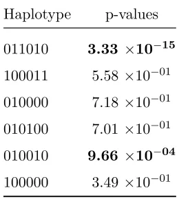
Table 2.1: Haplotype Specific Testing Example: Reference haplotype=100010
Haplotype p-values
011010 3.33 ×10⁻¹⁵
100011 5.58 ×10−01 010000 7.18 ×10−01 010100 7.01 ×10−01 010010 9.66 ×10−04
100000 3.49 ×10−01
011010 as the reference haplotype and tested the relative effects of the others. The results from these tests are in Table 2.2. From these results alone, we could only divide the haplotypes into 2 groups, one containing haplotype 011010 and one containing the remaining haplotypes. These results would be misleading because we would not be able to distinguish haplotype 010010 from the group of remaining haplotypes. But putting these results together with those from using haplotype 100010 as a reference, we can conclude that 011010 and 010010 are both different from all of the others and different from each other. If we carry out the remaining pairwise comparisons, shown in Table 2.3, we then have the complete picture of the relationships between all of the haplotype clusters.
Table 2.2: Haplotype Specific Testing Example: Reference haplotype=011010
Haplotype p-values
100010 1.34 ×10⁻¹⁰
100011 6.41 ×10−06
010000 6.20 ×10−06
010100 5.77 ×10−09
010010 1.92 ×10−04
100000 1.60 ×10−06
Table 2.3: Haplotype Specific Testing Example: Remaining Comparisons
Reference Haplotype p-values
100011 010000 8.88×10−01 010100 5.54×10−01 010010 3.50 ×10−02
100000 2.87×10−01 010000 010100 6.77×10−01 010010 3.30 ×10−02
100000 4.14×10−01 010100 010010 2.37 ×10−02
to the reference while conditioning on the effects of the other haplotypes. We choose to include separate terms for all of the core haplotypes in our model, but then col-lapse these haplotypes together if appropriate according to the results of the haplotype specific tests.
When we conduct all possible pairwise haplotype specific comparisons, we must control the familywise error rate by adjusting for multiple comparisons. We use the Bonferroni correction method, which adjusts the α level by dividing by the number of comparisons being made. The Bonferroni method is a conservative method that is easy to implement. In the example above, if the original α level was 0.05, we would declare a comparison significant if the p-value is less than 0.05/21=0.002.
2.3
Simulations
2.3.1
Scenarios
To assess the size and power of the proposed score tests, we simulated data using two different scenarios. We will describe the coalescent simulation and the FUSION simulation.
Coalescent Simulation
This says that the odds of disease for one copy of the liability allele are 1.6 times the odds for zero copies of the liability allele. We set b2 = 0.3 and let b0 range from -3.0 to -3.3, depending on the frequency of the liability locus. These parameter values were chosen so that the disease prevalence would be approximately 5 % for each scenario.
To evaluate the haplotype specific test, we chose a high haplotype diversity region with 10 haplotypes. We generated data assuming 2 different liability haplotypes with frequencies 0.12 and 0.08. For 2 liability haplotypes, the penetrance functionfjikis the probability that an individual is a case given they have j copies of liability haplotype 1, k copies of liability haplotype 2, and level i of a binary environmental covariate. The model at the liability haplotypes becomes logit(fjik) = b0 +b1j +b2k+b3i. To evaluate power, we generated data assuming the 2 liability haplotypes had the same effect (b1 = b2 = 0.5) and also assuming they had different effects (b1 = 0.7, b2 = 0.5 and b1 = 0.7, b2 = 0.3). We set b3 = 0.3 and varied b0 to achieve a 5 % disease prevalence.
FUSION Simulation
01100 as the causal haplotype, as Epstein and Satten (2003) found this haplotype to increase the risk of Type II diabetes using their retrospective approach. We simulated the haplotype data and binary environmental covariate for each individual conditional on disease status. We assumed haplotype-environment independence and HWE for simulating control data. For case subjects, we used the model
P(H = (h, h′), E =e|D= 1) = exp(XChh′β+Xeγ)phph′F0(e)
P
H
P
e∗exp(XChh′β+Xe∗γ)phph′F0(e
∗), (2.5)
where F0(e) is the probability of having covariatee in controls. Based on the FUSION results, we set F0(0) = 0.17, F0(1) = 0.83, and γ = 1.39. To evaluate Type I error, we set β01100 = 0.0, and evaluated power for β01100 = 0.2 and β01100 = 0.4. We also used the same sample size as the FUSION study: 727 cases and 415 controls. To evaluate the haplotype specific test, we set β01100 = 0.5.
For the global haplotype test, we simulated 2000 datasets to assess Type I error and 1000 datasets to assess power for α = 0.05 and α = 0.01 for both simulation scenarios. We also conducted the analyses using the retrospective, full-dimensional approach, and the prospective full-dimensional and clustering approaches on the same datasets for both simulations.
Table 2.4: Type I error rate for Coalescent Simulation: Global Haplotype Test (α= 0.05)
Hap Diversity RD retro FD retro RD prosp FD prosp
High:
q=0.1 0.048 (0.005) 0.044 (0.005) 0.050 (0.005) 0.050 (0.005)
q=0.3 0.043 (0.005) 0.047 (0.005) 0.046 (0.005) 0.051 (0.005)
Moderate:
q=0.1 0.047 (0.005) 0.028 (0.004) 0.052 (0.005) 0.051 (0.005)
q=0.3 0.040 (0.004) 0.023 (0.003) 0.041 (0.004) 0.049 (0.005)
Low:
q=0.1 0.054 (0.005) 0.044 (0.005) 0.052 (0.005) 0.047 (0.005)
q=0.3 0.046 (0.005) 0.039 (0.004) 0.045 (0.005) 0.045 (0.005)
RD denotes reduced-dimensional (or clustering) analysis. FD denotes
full-dimensional analysis. Retro denotes retrospective analysis. Prosp
denotes prospective analysis. Numbers in parentheses are Monte Carlo
standard deviations.
is a large number of estimated haplotypes. The prospective full-dimensional method can be carried out using haplo.glm in R, but we did not use this method as it is not comparable to the retrospective clustering method.
2.3.2
Results
Coalescent Simulation
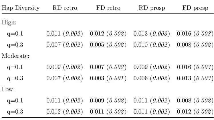
Table 2.5: Type I error rate for Coalescent Simulation: Global Haplotype Test (α= 0.01)
Hap Diversity RD retro FD retro RD prosp FD prosp
High:
q=0.1 0.011 (0.002) 0.012 (0.002) 0.013 (0.003) 0.016 (0.003)
q=0.3 0.007 (0.002) 0.005 (0.002) 0.010 (0.002) 0.008 (0.002)
Moderate:
q=0.1 0.009 (0.002) 0.007 (0.002) 0.009 (0.002) 0.016 (0.003)
q=0.3 0.007 (0.002) 0.003 (0.001) 0.006 (0.002) 0.013 (0.003)
Low:
q=0.1 0.011 (0.002) 0.009 (0.002) 0.011 (0.002) 0.008 (0.002)
q=0.3 0.012 (0.002) 0.011 (0.002) 0.011 (0.002) 0.012 (0.002)
RD denotes reduced-dimensional (or clustering) analysis. FD denotes
full-dimensional analysis. Retro denotes retrospective analysis. Prosp
denotes prospective analysis. Numbers in parentheses are Monte Carlo
standard deviations.
controls. The Type I error rate for the global tests for main haplotype effects are close to the nominal level for each of the analyses. This is evidence that the χ2 distribution accurately approximates the asymptotic distribution of the score statistics.
Table 2.6: Power for Coalescent Simulation: Global Haplotype Test (α= 0.05)
Hap Diversity RD retro FD retro RD prosp FD prosp
High:
q=0.1 0.849 (0.011) 0.775 (0.013) 0.843 (0.012) 0.772 (0.013)
q=0.3 0.646 (0.015) 0.639 (0.015) 0.644 (0.015) 0.639 (0.015)
Moderate:
q=0.1 0.562 (0.016) 0.479 (0.016) 0.560 (0.016) 0.504 (0.016)
q=0.3 0.911 (0.009) 0.844 (0.011) 0.907 (0.009) 0.868 (0.011)
Low:
q=0.1 0.839 (0.012) 0.827 (0.012) 0.835 (0.012) 0.826 (0.012)
q=0.3 0.796 (0.013) 0.779 (0.013) 0.798 (0.013) 0.778 (0.013)
RD denotes reduced-dimensional (or clustering) analysis. FD denotes
full-dimensional analysis. Retro denotes retrospective analysis. Prosp
denotes prospective analysis. Numbers in parentheses are Monte Carlo
standard deviations.
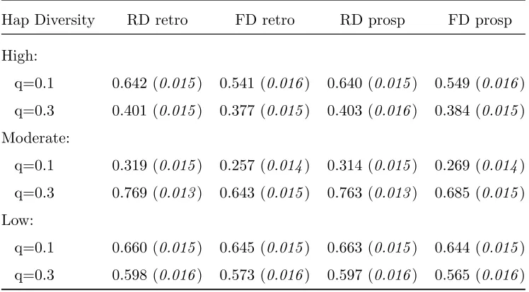
Table 2.7: Power for Coalescent Simulation: Global Haplotype Test (α= 0.01)
Hap Diversity RD retro FD retro RD prosp FD prosp
High:
q=0.1 0.642 (0.015) 0.541 (0.016) 0.640 (0.015) 0.549 (0.016)
q=0.3 0.401 (0.015) 0.377 (0.015) 0.403 (0.016) 0.384 (0.015)
Moderate:
q=0.1 0.319 (0.015) 0.257 (0.014) 0.314 (0.015) 0.269 (0.014)
q=0.3 0.769 (0.013) 0.643 (0.015) 0.763 (0.013) 0.685 (0.015)
Low:
q=0.1 0.660 (0.015) 0.645 (0.015) 0.663 (0.015) 0.644 (0.015)
q=0.3 0.598 (0.016) 0.573 (0.016) 0.597 (0.016) 0.565 (0.016)
RD denotes reduced-dimensional (or clustering) analysis. FD denotes
full-dimensional analysis. Retro denotes retrospective analysis. Prosp
denotes prospective analysis. Numbers in parentheses are Monte Carlo
standard deviations.
Table 2.8: Type I error Rate and Power for Coalescent Simulation: Haplotype Specific Test (α= 0.05)
True Effect Global Hap1 Hap2
β1=β2=0.0 0.039 (0.006) 0.025 (0.005) 0.029 (0.005)
β1=β2=0.5 0.958 (0.009) 0.892 (0.014) 0.794 (0.018)
β1=0.7,β2=0.3 0.994 (0.003) 0.998 (0.002) 0.312 (0.021)
β1=0.7,β2=0.5 0.998 (0.002) 1.000 (<0.001) 0.798 (0.018)
Table 2.9: Type I error Rate and Power for Coalescent Simulation: Haplotype Specific Test (α= 0.01)
True Effect Global Hap1 Hap2
β1 =β2=0.0 0.007 (0.003) 0.005 (0.002) 0.003 (0.002)
β1 =β2=0.5 0.854 (0.016) 0.716 (0.020) 0.556 (0.022)
β1=0.7,β2=0.3 0.976 (0.007) 0.988 (0.005) 0.120 (0.015)
β1=0.7,β2=0.5 0.990 (0.004) 0.980 (0.006) 0.570 (0.022)
Numbers in parentheses are Monte Carlo standard deviations.
average dimension reduction of 3. For the locus with frequency 0.3 in a moderate haplotype diversity region, there was an average of 14 observed haplotypes and an average dimension reduction of 4.
Table 2.10: Type I Error Rate and Power for FUSION Simulation: Global Haplotype Test (α= 0.05)
True Effect RD retro FD retro RD prosp FD prosp
β=0.0 0.050 (0.005) 0.032 (0.004) 0.051 (0.005) 0.060 (0.005)
β=0.2 0.255 (0.014) 0.158 (0.012) 0.248 (0.014) 0.188 (0.012)
β=0.4 0.865 (0.011) 0.724 (0.014) 0.834 (0.012) 0.649 (0.015)
RD denotes reduced-dimensional (or clustering) analysis. FD denotes
full-dimensional analysis. Retro denotes retrospective analysis. Prosp
denotes prospective analysis. Numbers in parentheses are Monte Carlo
standard deviations.
0.3, both the global haplotype test and the test for causal haplotype 1 have very high power. Causal haplotype 2 has a smaller frequency and effect size, and therefore there is lower power to detect the effect of this haplotype.
FUSION simulation
analy-Table 2.11: Type I Error Rate and Power for FUSION Simulation: Global Haplotype Test (α= 0.01)
True Effect RD retro FD retro RD prosp FD prosp
β=0.0 0.010 (0.002) 0.004 (0.001) 0.010 (0.002) 0.021 (0.003)
β=0.2 0.116 (0.010) 0.048 (0.007) 0.110 (0.010) 0.066 (0.008)
β=0.4 0.676 (0.015) 0.488 (0.016) 0.637 (0.015) 0.436 (0.016)
RD denotes reduced-dimensional (or clustering) analysis. FD denotes
full-dimensional analysis. Retro denotes retrospective analysis. Prosp
denotes prospective analysis. Numbers in parentheses are Monte Carlo
standard deviations.
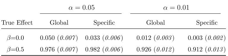
Table 2.12: Type I Error Rate and Power for FUSION Simulation: Haplotype Specific Test
α= 0.05 α = 0.01
True Effect Global Specific Global Specific
β=0.0 0.050 (0.007) 0.033 (0.006) 0.012 (0.003) 0.003 (0.002)
β=0.5 0.976 (0.007) 0.982 (0.006) 0.926 (0.012) 0.912 (0.013)
Numbers in parentheses are Monte Carlo standard deviations.
ses. This indicates that the score statistics under H0 have the proper χ2 asymptotic distribution. The full-dimensional retrospective test is slightly conservative, which can be expected because of the large number of degrees of freedom. The full-dimensional prospective test is slightly anti-conservative.
sizes, and has slightly greater power than the clustering prospective analysis. For both retrospective and prospective approaches, the clustering analysis has greater power than the full-dimensional analysis. This difference in power is similar for the retrospec-tive and prospecretrospec-tive approaches.
The haplotype specific test results are presented in Table 2.12. As with the coales-cent simulation, the haplotype specific test is conservative. The global and specific tests have almost identical power, which is expected as there is only one causal haplotype. Therefore the global and specific tests are detecting the same effect.
2.4
Conclusions
We have proposed a method that addresses one of the major limitations to the useful-ness of haplotype analysis for detecting genetic associations in complex diseases. Our method reduces the degree of freedom by clustering haplotypes and carrying out infer-ence based on a core set of haplotypes. The method uses unphased genotype data and can incorporate environmental covariates, which is important when studying complex diseases. The method has greater power than the retrospective full-dimensional ap-proach, evidence that reducing the degrees of freedom through clustering improves the performance of haplotype analysis. The greater the dimension reduction due to clus-tering, the larger the difference in power between the clustering and full-dimensional approaches. This can be seen from the larger power difference in our results from the FUSION simulation, where the dimension reduction is much greater than for any of the coalescent simulation scenarios.
clustering approaches. This supports the finding of Satten and Epstein (2004) that retrospective and prospective likelihood analyses have similar power when assuming haplotypes have a multiplicative effect on the disease odds. Our clustering retrospec-tive likelihood assumes a multiplicaretrospec-tive model of disease odds because the clustering algorithm must make this assumption.
The clustering retrospective method assumes a rare disease, while the clustering algorithm is based on the common disease/common variant hypothesis. The com-mon disease/comcom-mon variant hypothesis says that comcom-mon variants are responsible for common diseases. This assumption for the clustering algorithm allows us to reduce the degrees of freedom by concentrating attention on common variants that comprise the set of core haplotypes. We do not expect this contradiction to be a problem as we expect rare causal variants to be oversampled in a case-control sample. In addi-tion, Kwee et al. (2007) found that the retrospective method assuming a multiplicative disease model is robust to the assumption of a rare disease. Case-control studies are usually used when the disease prevalence is less than 10 %, and they found the method has similar size and power for disease prevalences of 5 % and 10 %.
Satten and Epstein (2004) also show that the retrospective approach with a mul-tiplicative model is robust to the assumption of HWE in the target population. They also propose a method to model departure from HWE due to inbreeding and population stratification by incorporating a fixation index. The fixation index is a measurement of how different the subpopulation is from a population in HWE.
Testing for Haplotype-Environment
Interactions
3.1
Introduction
allows us to incorporate these assumptions and improve efficiency.
Some of the retrospective methods presented in Chapter 1 only present tests to test for interaction between a specific haplotype and the covariate of interest. While there are situations where this may be an appropriate test to consider, ideally we would use the same strategy to study interaction effects that we use for studying main effects. We wish to first carry out a global test for interaction effects. Then if a global association is detected, we carry out tests for specific interaction effects. This strategy is usually not practical for methods that consider the full-dimensional haplotype space due to lack of power from large degrees of freedom. But our method uses a reduced set of haplotypes, and therefore this strategy becomes feasible.
3.2
Methods
3.2.1
The Retrospective Likelihood for Haplotype-Environment
Interaction
Here we extend the likelihood in (2.3) to allow for haplotype-environment interactions. We write the design matrix for haplotype-environment interactions asXC⊗XE, where
⊗ denotes the Kronecker product. If we assume a binary covariate, we write the row of the design matrix corresponding to haplotype pair H as
XHE =XCH ⊗XE =
XCH1XE XCH2XE . . . XCHL∗XE.
XHE will haveL∗(k−1) columns, wherek is the number of levels of the environmental covariate and (L∗ + 1) is the number of haplotype clusters. We write the vector of
L∗(k−1) interaction parameters as ν. We can modify the odds of disease as
θ(H, E) = exp(α+XCβ+XEγ+XHEν)
and now the likelihood for testing for interactions becomes
Lobs ∝ n
Y
i=1
P
H∈S(Gi)exp(α
∗+XC
Hβ+XEiγ+XHEiν)phph′
1 +θ∗(E
i)
di P
H∈S(Gi)phph′
1 +θ∗(E
i)
1−di
.
3.2.2
Score Test for Global Interaction Effect
The null hypothesis to test for global interaction effects for a certain environmental covariate is H0 :ν = 0. The score statistic is Sν =UνTVν−1Uν
ν
=0,ξ=ξ˜
, and has a χ2 distribution with L∗(k−1) degrees of freedom.
Uν = ∂
∂ν logLobs
and
Vν =Dνν −IνξIξξ−1DνξT −DνξIξξ−1IνξT +IνξIξξ−1DξξIξξ−1IνξT ,
where D is the variance-covariance matrix of the score function U = (Uν,ξ)T and I is the observed information matrix (Boos (1992)). The vector of nuisance parameters, ξ, now consists of α∗,γ, β, andp. See Appendix B for detailed expressions for the score
and variance functions.
Estimation
3.2.3
Score Test for Specific Haplotype-Environment
Interac-tion Effect
The test for a specific interaction effect tests the hypothesis that the specific effect is 0 while the other interaction effects are unconstrained. If we include one covariate in the model, the null hypothesis for testing for an interaction between haplotype t and the covariate is H0 :νt= 0. The score function is
Uνt =
∂ ∂νt
logLobs
and the generalized variance function is
Vνt =Dνtνt−IνtξI
−1
ξξD
T
νtξ −DνtξI
−1
ξξI
T
νtξ+IνtξI
−1
ξξDξξI
−1
ξξI
T νtξ.
The score statistic is Sνt =U
T νtV
−1 νt Uνt
νt=0,ξ=ξ˜
, and has aχ2 distribution with 1 degree of freedom. The vector of nuisance parameters ξ now contains α∗, β, γ, p, and the
interaction parameters ν, excluding νt.
Estimation
E Step
The E step for estimating the number of controls with haplotype pair (h, h′) and
covariate level k is the same as that in Section 2.2.3. The E step for estimating the number of cases with haplotype pair (h, h′) and covariate level k is now
E(dhh′,k) =
X
g
dg,kI(H ∈S(g))P(H|g)
=X
g
dg,kI(H ∈S(g))
exp(α∗+X
CHβ+XEkγ+XHEkν)phph′
P
H∈S(g)exp(α∗+XCHβ+XEkγ+XHEkν)phph′
M step 1: Estimating p
To estimate p, we use a Lagrange multiplier λ and maximize the log of the full-data likelihood subject to the constraint P
hph = 1.
LM = logLf ull+λ(
X
h
ph−1) =
e
X
k=1
X
(h,h′)
chh′,klog(phph′) +dhh′,k[(α∗+XC
hh′β+XEkγ+X(h,h′)Ekν)+
log(phph′)]−log(1 +
X
H
exp(α∗+XCHβ+XEkγ+XHEkν)phph′)
(chh′,k +dhh′,k)
+λ(X h
ph−1) =
e
X
k=1
X
(h,h′)
chh′,klog(phph′) +dhh′,k[(α∗+XC
hh′β+XEkγ+X(h,h′)Ekν)+
log(phph′)]−log(1 +
X
H
exp(α∗+XCHβ+XEkγ+XHEkν)phph′)
(chh′,k +dhh′,k)
+λ(X h
ph−1) =
e
X
k=1
X
(h,h′)
log(phph′)(chh′,k+dhh′,k) +dhh′,k(α∗+XC
hh′β+XEkγ+X(h,h′)Ekν)−
nhh′,klog(1 +
X
H
exp(α∗+XCHβ+XEkγ+XHEkν)phph′)
+λ(X h
The portion of LM that depends on p is
LM ∝ e
X
k=1
X
(h,h′)
log(phph′)nhh′,k− nhh′,klog(1 +
X
H
exp(α∗+XCHβ+XEkγ+XHEkν)phph′)
+λ(X h
ph −1)
∝ e X k=1 X h
mh,klog(ph)
− e X k=1 X
(h,h′)
nhh′,klog(1 +
X
H
exp(α∗+XCHβ+XEkγ+XHEkν)phph′)
+λ(X h
ph−1),
wheremh,k is the number of haplotypes of typehwith covariate levelk. The derivative with respect to a specific pτ is
∂ ∂pτ
LM ∝ e X k=1 mτ,k pτ − e X k=1 X
(h,h′)
nhh′,k
P
Hexp(α∗+XCHβ+XEkγ+XHEkν)I(h=τ)2ph′
1 +P
Hexp(α∗+XCHβ+XEkγ+XHEkν)phph′
+λ ∝ e X k=1 mτ,k pτ − e X k=1 nk P
h′exp(α
∗ +X
Cτ,h′β+XEkγ+X(τ,h′)Ekν)2ph′
1 +P
H exp(α∗ +XCHβ+XEkγ+XHEkν)phph′
+λ.
As in Chapter 2, we define the quantity u(p)τ as
u(p)τ = e
X
k=1 nk
P
h′exp(α∗+Xτ,h′β+XEkγ+X(τ,h′)Ekν)2ph′
1 +P
where nk is the number of subjects with covariate level k. Then the derivative with respect to pτ becomes
∂ ∂pτ
LM ∝ e
X
k=1 mτ,k
pτ
−u(p)τ +λ and the updating equation for pτ is
pτ =
Pe
k=1mτ,k (u(p)τ −λ)
. (3.2)
We carry out another iteration within the M step for estimating p by estimating u(p)(s,k) based on p(s), then estimating p(s,k+1) based on u(p)(s,k). This iteration con-tinues until the difference betweenp(s,k)andp(s,k+1) is less than a specified limit. Then p(s,k+1) becomesp(s+1).
M step 2: Estimating α∗, γ, β, and ν
The log of the full likelihood that depends on the regression parameters is
logLf ull ∝ e
X
k=1
X
(h,h′)
−nhh′,klog(1 +
X
H
exp(α∗+XCHβ+XEkγ+XHEkν)phph′)
+dhh′,k
log(exp(α∗+XCHβ+XEkγ+XHEkν)) + logphph′
∝
e
X
k=1
X
(h,h′)
−nhh′,klog(1 +
X
H
exp(α∗+XCHβ+XEkγ+XHEkν)phph′)
+dhh′,k(α∗+XCHβ+XE
kγ+XHEkν).
We obtain maximum likelihood estimates for α∗, β, γ, and ν using the optimization
3.3
Simulations
3.3.1
Scenarios
To assess the size and power of the proposed score tests for interactions, we use simu-lation scenarios similar to those described in Chapter 2.
Coalescent Simulation
The coalescent simulation uses haplotype data generated using the coalescent model. We perform case-control sampling and use a single SNP as the disease liability locus. We use the same 6 scenarios for selecting a disease locus as in Chapter 2, which are chosen based on allele frequency (0.1 and 0.3) and haplotype diversity (high, moderate, and low) in the region. The logistic model for the liability variant allows for the effect of an interaction between the liability variant and the environmental covariate, and is defined as logit(fji) = b0 +b1j +b2i+b3i∗j where j is the number of copies of the liability SNP and i is the level of the environmental covariate. We set b3 = 0.0 to evaluate Type I error rate and b3 = 0.5 and 0.7 to evaluate power. We set b1 = 0.5, b2 = 0.3, and vary b0 so that the prevalence for each situation is approximately 5 %. We analyze 6-SNP haplotypes that exclude the liability locus. The haplotypes are formed from the 3 adjacent SNPs directly to the left and right of the liability locus. For each replicate we generate 500 cases and 500 controls.
fjik is the probability that an individual is a case given they have j copies of liability haplotype 1, k copies of liability haplotype 2, and level i of the binary environmental covariate. We evaluated power assuming the interaction effects between both of the liability haplotypes and the covariate were the same (b4 = b5 = 0.5) and different (b4 = 0.7, b5 = 0.5). We set b1 = b2 = 0.5, b3 = 0.3, and varied b0 to achieve a 5 % disease prevalence.
FUSION Simulation
The FUSION simulation uses haplotype data based on 5 SNPs of interest on chromo-some 22 in the FUSION study. We allow for interaction between the causal haplotype (01100) and the environmental covariate by modifying equation (2.5) to become
P(H = (h, h′), E =e|D= 1) = exp(XChh′β+Xeγ+Xhh′,eν)phph′F0(e)
P
H
P
e∗exp(XChh′β+Xe∗γ+Xhh′,e∗ν)phph′F0(e
∗).
(3.3) We set the probability for each level of the covariate in the controls to be 0.5. This eliminates estimation problems that could result from having low counts for certain haplotype-environmental covariate combinations. We used the same sample size as in scenario 1: 500 cases and 500 controls. We setβ01100= 0.65,γ = 1.39, andν01100,1 = 0.0 to evaluate Type I error rate and ν01100,1 = 0.3, 0.5, and 0.7 to evaluate power. We evaluated the interaction specific test using the simulated data with an effect size of 0.7.
dimensional method of Kwee et al. (2007). For this analysis, we must estimate the full-dimensional main effect parameters. In the case of the interaction specific test, we must estimate all of the full-dimensional interaction parameters except the one that is being tested. Therefore the estimation for these parameters of main and interaction effects is not feasible for the FUSION simulation and the high and moderate haplotype diversity regions of the coalescent simulation. Furthermore, there is no available interaction test for the prospective clustering method. Consequently, in this chapter we will evaluate our proposed test under the retrospective framework, and report the results of the clustering analysis only for most scenarios.
3.3.2
Results
Coalescent Simulation
Table 3.1 presents the Type I error rate analysis for the global interaction test from the coalescent simulation. The Type I error rate is at the nominal level for all six of the liability loci for the global interaction test, indicating that the χ2 distribution accurately estimates the asymptotic distribution of the score statistic.
Table 3.1: Type I Error Rate for Coalescent Simulation: Global Interaction Test
α = 0.05 α= 0.01
Hap Diversity RD retro FD retro RD retro FD retro
High:
q=0.1 0.054 (0.007) NA 0.015 (0.004) NA
q=0.3 0.048 (0.007) NA 0.010 (0.003) NA
Moderate:
q=0.1 0.056 (0.007) NA 0.010 (0.003) NA
q=0.3 0.067 (0.008) NA 0.014 (0.004) NA
Low:
q=0.1 0.057 (0.007) 0.042 (0.006) 0.009 (0.003) 0.008 (0.003)
q=0.3 0.047 (0.007) 0.038 (0.006) 0.014 (0.004) 0.011 (0.003)
RD denotes reduced-dimensional (or clustering) analysis. FD denotes
full-dimensional analysis. Retro denotes retrospective analysis. NA
indicates that the analysis was not conducted. Numbers in parentheses
are Monte Carlo standard deviations.
full-dimensional analysis. The retrospective full-dimensional analysis is only feasible in regions with low haplotype diversity. As with the test for global main haplotype effects, we do not expect a large difference in power between the clustering and full-dimensional analyses for low haplotype diversity regions since the reduction in degrees of freedom is small. We are still able to observe slight power improvement. This result suggests potential power gain that can be brought by the clustering strategy when the haplotype diversity is moderate and high.
Table 3.2: Power for Coalescent Simulation: Global Interaction Test,ν = 0.5
α= 0.05 α = 0.01
Hap diversity RD retro FD retro RD retro FD retro
High:
q=0.1 0.422 (0.022) NA 0.222 (0.019) NA
q=0.3 0.188 (0.017) NA 0.060 (0.011) NA
Moderate:
q=0.1 0.240 (0.019) NA 0.088 (0.013) NA
q=0.3 0.262 (0.020) NA 0.110 (0.014) NA
Low:
q=0.1 0.496 (0.022) 0.420 (0.022) 0.244 (0.019) 0.208 (0.018)
q=0.3 0.280 (0.020) 0.264 (0.020) 0.104 (0.014) 0.084 (0.012)
RD denotes reduced-dimensional (or clustering) analysis. FD denotes
full-dimensional analysis. Retro denotes retrospective analysis. NA
indicates that the analysis was not conducted. Numbers in parentheses
are Monte Carlo standard deviations.