A feedback control algorithm for a second-order dynamic system

VICTORIA ~ UNIVERSITY

.

•

.

....

~

"· .· 0 ~ 0 ···· ... ··.

:

DEPARTMENT OF COMPUTER AND

MATHEMATICAL SCIENCES

A Feedback Control Algorithm for a

Second-order Dynamic System

Venkatesan Gopalachary

(64 EQRM 19)

December, 1995

(AMS: 60G99)

TECHNICAL REPORT

VICTORIA UNIVERSITY OF TECHNOLOGY

DEPARTMENT OF COMPUTER AND MATHEMATICAL SCIENCES

P 0

BOX 14428

MCMC

MELBOURNE, VICTORIA 8001

AUSTRALIA

TELEPHONE (03) 9688 4492

FACSIMILE (03) 9688 4050

A FEEDBACK CONTROL ALGORITHM FOR A

SECOND-ORDER DYNAMIC SYSTEM

Venkatesan Gopalachary,

Victoria University of Technology, Melbourne, Australia.

Abstract

Statisticians and control engineers, often taking different perspectives, have long practised the 'art' of

process control. In recent years, attention has been focussed on bringing the two control

methodologies closer together. This report addresses some of the issues of automatic process control,

with specific reference to continuous processes, such as stability of the feedback control path and the

existence of dead time. A method to derive a control algorithm for making an adjustment that would

yield the smallest possible mean square error (variance) of the output controlled variable is given for

the critically damped second-order dynamic system.

1 INTRODUCTION

In manufacturing processes, uniform outputs are generally not attainable due to factors which

cause unpredictable variation. The presence of non-random causes in a production system, (an

assignable cause), may be detected as an unexpected variation in the system measurements.

'Disturbances' may afflict the system causing it to drift off target if no action is taken to eliminate

them. A requirement for a process to be controlled satisfactorily is that its output should follow both

some reference signal and remain unaffected by extraneous disturbances or parameter variations.

Engineering control systems continually adjust processes on-line in an attempt to counteract the

effects of disturbances. Statistical process control (SPC) aims to contain variation in output so that

attempt to reduce variability. Automatic process control aims to maintain certain key process

variables as near their desired values called set points for as much of the time as possible in order to

satisfy production objectives. One approach is to forecast the deviation from target which would

occur if no action were taken and then act so as to cancel out this deviation. In this report, an

explanation is given to how a stochastic model can be used to describe the effects of disturbances and

to develop a feedback control algorithm.

2 PROCESS CONTROL

Global production objectives are to achieve production targets at an acceptable cost and to

manufacture products of a desired quality in a safe manner with the minimum possible harm to the

environment. These goals are realised by monitoring and controlling production. Control tools are

used:

(i)

(ii)

to detect changes in process performance from a stable state,

to identify assignable or special causes of variation indicated by

these deviations and eliminate the same and/or

(iii) to adjust a process variable or variables so as to maintain a performance criterion in

some desirable neighbourhood of a given target value (Box and Jenkins [1963]).

The first two control actions of process monitoring and control are achieved by statistical

process control (SPC) techniques. The third process control action is possible by an appropriate

feedback or feedforward control procedure which indicates when and by how much to adjust the

process automatically, by either using the deviation from target of the output or by cancelling these

deviations by using knowledge of the value of some fluctuating measured input variable,

Use of automatic control began in the late 1920's and the first technical publication appeared

in 1932. Since then, there has been a steady growth in and use of automatic control systems. Various

forms of feedback and feedforward control regulation schemes are used for process adjustment

(control action) in automatic process control (APC). APC provides an instantaneous continuous

response counteracting changes in the balance of a process and applying self-corrective action to

bring the output close to the desired target often without human intervention (Keats and Hubele

[1989]).

The term 'controlled process' is often used to mean a 'process state' that is (narrowly)

interpreted as stationary having iid variation about a target value. An alternative has a 'state of

control' as a process state in which future behaviour can be predicted within probability limits

determined by a common-cause system (Box and Kramer [1992]).

If a state of statistical control is identified by a process generating independent and identically

distributed (iid) random variables, control of such random processes by automatic means invariably

leads to an undesirable increase in process variability. APC provides a consistent steady dynamic

response in counteracting changes in the balance of a process and must be properly applied to obtain

successful results.

In situations where the cost of making an adjustment to the process is considerable, APC can

result in increased cost. In comparison with SPC, APC, referred to as 'engineering feedback control'

is a short-term approach that attempts to minimise (output) variation by transferring the predictable

component of the output variation to the input manipulated (control) variable [MacGregor] (Box and

Kramer [1992]). The appropriate engineering control strategy depends upon (i) the characteristics of

the stochastic (statistical) component of the process modelled by a suitable time series and (ii) the

The general purpose of automatic control is to get satisfactory process operation by

adjustment of a controller (control mechanism). By using a logical method for selecting controller

adjustments and by suitable 'tuning', (which means, to have the freedom of choice to vary the

parameters of control), there is the potential for high returns in the form of efficient process

operation. By suitably modelling a process that is non-stationary but probabilistically predictable, it

is possible to formulate a control mechanism leading to the 'adaptive control' situation (Box and

Jenkins [1970, 1976]).

3 STOCHASTIC MODELS AND STOCHASTIC DISTURBANCES

In process control, it is common to come across disturbances (noise) that are drifting or

nonstationary in nature. The importance of considering disturbances of this nature was known to

control system engineers from the early stages of the development of deterministic control theory.

Deterministic control theory was developed to provide tools to analyse and synthesise a large variety

of feedback control systems. Results from various branches of applied mathematics and control

problems were used in developing this theory. The early development focussed on stability theory

and the theory of analytic functions. Due to complexity and the stringent performance criteria

required of controlled processes, the theory of optimal control of deterministic processes was

developed using the tools of the calculus of variations. In controlling deterministic processes, no

significant distinction was made between a feedback control system and a feedforward control

system and no dynamics (inertia) was assumed in the feedback. There were some drawbacks in using

deterministic control theory such as not using realistic models for disturbances and when a

disturbance was introduced, it was postulated as a function which is known a priori. Many of the

[1956]). The effects of disturbances were required to be predicted by suitable models and there

existed the need to model the disturbances in a proper and fitting manner.

Since analytic functions are limited in their capacity to accurately model, the potential for the

use of 'statistical models' became apparent. Barnard [1959] and Bather [1963] linked the control

problem and SPC charts. Barnard [1959] suggested that for a wandering industrial process, by using

control charts and its signals, improvements in process adjustments can be made by means of a

model that c!osely described the disturbance and an estimate of the current process mean connected

with the control problem. Other statisticians, Box [1970], Jenkins [1970] and Astrom [1970]

endeavoured to provide an answer to the problem of how to characterise and model the disturbance.

A 'deterministic model' makes possible exact calculation of the value of some time-dependent

quantity at any instant of time. In many process control problems, unknown factors make this

unrealistic. However, it is often possible to derive a realistic model that can be used to calculate the

probability of a future value lying between two specified limits. Such a model is called a

'probabilistic' or a 'stochastic model'. Box and Jenkins [1970,1976] adopted this approach and made a

major contribution to stochastic control.

Since a disturbance causes a process to drift off target, it is necessary to compensate this by

taking proper control action. A process in which the mean is varying in nature with respect to time

can be described as a non-stationary disturbance. A stationary disturbance represents the situation

where there is no drift in the mean and the process is in a perfect state of control.

Disturbances entering at various points of a process are often persistent in nature, however, in

many instances, it may not be economically possible or physically feasible to eliminate them. Such

disturbances can be envisaged as the result of a sequence of independent random shocks which can

be represented by a first order differential equation, such a system being referred to as a 'first-order

Control systems engineers described the system model behaviour in which the response of a

system to a given input is certain and well defined (deterministic). They used (linear) differential

equations to represent the dynamic (feedback) control systems in continuous time and used Laplace

transforms to obtain simplified solutions (Deshpande and Ash [1981]. The linearity assumption

supplies an approximation for many practical situations. In a similar manner, in dealing with discrete

processes, linear difference equations were employed to represent the processes in which the

sampling intervals are short enough so that the dynamic or inertial properties of the process cannot be

ignored. A first-order process may be represented by the first-order difference equation when

sampled at discrete intervals or by the first-order transfer function or 'filter', (the term used in

engineering terminology, by control system engineers), (cf. MacGregor [1987]).

Box and Jenkins [1965] set up realistic and flexible stochastic models for the disturbances

which force the system, unless controlled, away from their optimal operating conditions. They used

process knowledge and took care of the inertia or the dynamics of the system which makes the

control actions, needed to combat these disturbances, more complex in nature. In doing so, they

found methods for estimating the unknown parameters in the models from process input-output data.

They also used the models, after fitting the parameters, to design control schemes. Box, Jenkins and

MacGregor [1974], describe how stochastic and (dynamic) transfer function models may be brought

together to design feedforward and feedback control schemes. They showed how the parameters in

the stochastic and dynamic models may be simultaneously estimated from measurements made in the

operating system.

4 FEEDFORW ARD AND FEEDBACK CONTROL MODELS

A feedforward control model is proposed when the major disturbances to a production system

either not known or cannot be measured. Making use of the available knowledge of the production

process and the serially occurring data (which are very likely correlated), it is often possible to build

stochastic models to realistically represent and model the disturbances. Box and Jenkins [1970]

expressed the process inputs and outputs in terms of time series and described the disturbances by

time series models in order to manipulate the system for control purposes.

Feedforward or open-loop control is used to eliminate the effect of some fluctuating

measured input by making an adjustment from direct calculation of its effect on the output. For a

specified target value of the output, the feedforward control model gives an estimate of the required

change to be made in the compensating variable to minimise the mean square error (sum of the

squared deviations between an output value and the target value). When the time series model

predicts an out-of-control signal for shifts in the mean of the quality deviations from target, changes

are made to the compensating variable to offset the effects of the predicted situation (Keats and

Hubele [1989]).

Feedback or closed-loop control uses past output deviations from target to determine a

process adjustment. This approach makes use of the error (difference between the output and the

target values) as the means of identifying changes to the input. Using time series analysis, the effect

of the disturbance in the absence of a control action is estimated and a dynamic model is developed

linking the input and the process output.

5 ARIMA MODELS

The class of stochastic time series nonstationary models, called Autoregressive Integrated

Moving Average (ARIMA) Models developed by Box and Jenkins [1970,1976] are used to describe

the stochastic disturbances to the system and provide a means of modelling disturbances and process

process disturbances when no control action is taken and describe the dynamic relationship between

the controlled variables (outputs) and the manipulated variables (control inputs). From these models,

a feedback control algorithm is derived which minimises the variance of the output controlled

variable at every sample point which exactly compensates for the forecasted disturbance. Models of

this kind are used in inventory control problems, in econometrics and to characterise certain

disturbances that regularly occur in industrial processes.

6 CONTROLLERS

6.1 Proportional Integral Derivative (PID) Controllers

In feedback control systems, the process adjustments (control actions) are performed either

manually or by automatic means through the use of 'controllers'. Often a digital computer connected

directly to the process accomplishes the execution of the control action by observing the system so

that the available data appears in discrete-time.

Slow changes are encountered in many chemical processes. Under such circumstances, it may

be adequate to monitor and take whatever control action is necessary at convenient time intervals.

For many automatic controllers, as soon as the measurements are made, the control actions are

initiated immediately. By means of the discrete data, the adjustments are made to bring the process

into a state of control. With the process data available, it is possible to control the mean square error

about the target by proportional-integral feedback control schemes (Box and Kramer [1992]).

The proportional plus integral (PI) controller makes a compensation (correction) (which lags

behind the trend, if any, in the disturbance) proportional to a (linear) combination of terms

involving the deviation and the integral of all the previous errors. A PI controller is a 'standard linear

controller'. A special case of such a controller is, regulation based on the control-modified EWMA

The proportional integral derivative (PID) controller is a modified form of the PI

controller in which an additional term involving the first derivative with respect to the time of the

error is included. This type of automatic control action makes a correction which is proportional to a

(linear) combination of (i) the first derivative of the current deviation ('the difference between value

of the output controlled variable and position of the final controller set point'), (ii) the deviation

itself and (iii) the integral of the deviations over all past history (Box and Kramer [1990]). PID

controllers, also known as three-term controllers, are automatic continuous time controllers. These

controllers (i) are not capable of providing tight control over processes in which the effect of an

adjustment is delayed until the following sample due to time taken to deliver material from the point

of adjustment to the sample point (called, the 'dead time'), (ii) tend to perform poorly unless

'detuned' in the face of dead times in order to take necessary action at each sampling instant (page

428, Harris, MacGregor & Wright [1982]), and (iii) are not suited for direct-digital (discrete) control.

PID controllers are also not capable of producing control actions that might be called for by a

minimum variance feedback controller (page 437, Box and Jenkins [1970,1976]). Controllers

employing stochastic characteristics to regulate production processes are called time · series

controllers. With time series controllers, it is possible to provide tight control of processes with dead

time and to provide minimum variance at the same time.

6.2 Time Series Controllers - Characteristics and features

Time series controllers are used in the chemical and process industries for regulating quality

variables measured at discrete time intervals. Their 'stochastic feedback control algorithms'1 _{are used}

to calculate a series of adjustments which compensate the disturbances. Recourse to ARIMA models

is made to forecast their drifting behaviour and the stochastic feedback control algorithm or equation

derived from these ARIMA models is computerised. Thus 'time series control algorithms' by

calculating a series of adjustments compensate for the disturbances by making an adjustment at every

sample point.

7 MINIMUM VARIAN CE CONTROL

A feedback control strategy to minimise the mean square of the output deviation (error) from

the target is by minimum mean square error or variance control. Minimum variance control is the

best possible control for processes described by linear functions with disturbances which can be

added together and treated as a single disturbance for purposes of mathematical analysis and

convenience. Its implementation may demand aggressive control much in excess of what is

(normally) required and so may not be practically desirable. However, minimum variance control

provides a convenient bound on achievable performance against which the performance of other

controllers may be compared. Such a basis is important in the context of deciding corrective control

actions. Harris [1989] described a technique to ascertain the best theoretically achievable feedback

control performance as measured by the output mean square error.

Time series controllers are capable of giving a minimum control error variance even when

there are dynamics (inertia) and delay in the process control system. It may be possible to restrict

sampling a process until an acceptable minimum of control error variance can be achieved by making

use of the time series controller's minimum variance control property and to minimise monitoring

8 DEVELOPMENT OF TIME SERIES MODELS

8.1 Feedback Control Difference Equation

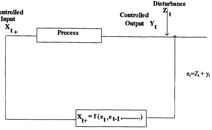
The 'stochastic difference equation' for the feedback control model is derived with the help of

a block diagram shown in figure 1.

Controlled Input

xt+ _Process

Disturbance

Controlled 1t Output Yt

'---~lxt+

11--~

Figure 1 Block Diagram for the Feedback Control Model

In the feedback control scheme shown in figure 1, the process is regulated by manipulating

the input variable Xt which in turn affects the controlled output Y t- Xt+ is the setting of the

controlled input variable (the plus sign on the subscript of Xt+ implies that the adjustment is made

during the interval between t and t+ 1 ). A definite deterministic relationship exists between the

process input X₁ and its output Y1 which does not exhibit stochastic characteristics. Z , the

non-t

stationary disturbance is the output of the (linear) system, when subjected to a sequence of

8.1.1 Symbols used in the Feedback Control model block diagram of figure 1.

2

~ Random shocks NID (0, a a),

Zt

et Forecast Error,

Xt+Input Manipulative Variable (Linear function of et and of integral over time of past errors),

Y t Output or Controlled Variable,

Box and Jenkins [1970,1976] described some dynamic models of the order (r,s) by

(Table 10.1, page 350, Box and Jenkins [1970,1976]), b being the number of whole periods of dead

time (delay), where

or(B) and os(B) are polynomials in Band BXt = Xt-1, Bbxt = Xt-b; Bis the backward shift operator.

A first-order single input single output (SISO) dynamic system is parsimoniously,

represented by the general (linear) difference equation

0::; 0 <1 (1)

where~= 0/1-o and \1 is the backward difference operator, \1=1-B.

The terms g(ain) and o are explained subsequently.

This discrete dynamic model of the order (r,s)

=

0::; 0 <1

Withs= 0, the impulse response tails off exponentially (geometrically) from the initial starting value

2 Note that we will be using 'z' to denote the stochastic variable and 'Z' to represent the stochastic

disturbance. The same logic holds good for at which denotes the variable and {at} represents the

roo

=

+

=

+

=

(page 352 Box and Jenkins [1970,1976]).

where g, the (steady-state) gain denotes the ratio of change in the steady-state process output to the

change in the input which caused it (Deshpande and Ash [1981], (Shinskey [1988]). 8 represents the

(dynamics) inertial capacity of a process to recover back to its equilibrium conditions after an

adjustment is made to the process and due to which the adjustments do not have an immediate effect

on the process. It is connected to the sampling interval and the time constant by means of the relation

8 = e-ttr where t is the sampling interval of the discrete process and T, the process time constant.

Time constant is the time required for the process output to complete 63 .2% of its final steady-state

value after a change is made in the input.

So, we write the recursive control equation for the first-order dynamic model with b

units of delay (dead time) in the form

(1-8B)Yt = rooXt-b = g(l-8)Xt-b

=

~

This is the feedback control first-order difference equation for the dynamic model for which the

output change asymptotically approaches 'g' for a unit change in the input, where 'g' is called also

the 'system' or 'pure' gain (Box and Kramer [1992]).

8.2 Justification For Second-Order Dynamic Models

For feedback control (closed-loop) stability, the parameter 8 must satisfy the condition

that O < 8 < 1 for the discrete dynamic model of the process and the gain should be less than or equal

to 1.0 (Shinskey [1988]).

The first-order dynamic model characterised by the linear difference equation (2) can

be written as

The MMSE (minimum mean square error) or minimum variance control schemes based on

the first-order dynamic model and the ARIMA (0, 1, 1) disturbance model produce the minimum

mean square error (MMSE) at the output requiring excessive control action in the following

situations in which (i) the values of 8 are not fairly small; and in (ii) as 8 becomes larger and in

particular, as it approaches unity (Box and Kramer [1992]). As 8 becomes larger, the minimum

variance control exhibits large 'alternating' character in the required adjustments (control actions) to

give minimum output variance (Box and Kramer [1992]). It is believed and understood that the

properties of the noise reflects the system inertia as well (Box and Jenkins [1970, 1976]).

For higher values of 8, the general recourse is to go in for constrained variance control

schemes. In such control schemes, reduced control action may be achieved at a cost of small

increases in the mean squared error at the output by placing a constraint on the input manipulated

variable. Kramer [1990] developed a constrained variance control scheme in which he showed the

effect on both adjustment variance and the specified output variance in order to evaluate the

trade-offs between the two variances.

The processes found in practice are complex because of their dynamic characteristics which

change with time. Approximating such processes by first-order dynamic models does not always

seem to be satisfactory. It can be shown from the simulation study results of the time series controller

for a first-order (plus dead time) dynamic model and ARIMA (0,1,1) model that for drifting

processes, for values of 8 from 0 to 1, the required adjustments are of alternating character and

sometimes with huge increases in control error standard deviation and its adjustment variance. It is

likely that some processes may have more than one dynamic element and the exact mathematical

model relating the output and the input could be greater than the first-order. Many complicated

dynamic systems can be fairly closely approximated to a greater extent by second-order systems with

system represented by a dynamic model of the order (2, i ), ('a discretely coincident' continuous

system, page 358, Box and Jenkins [i970,i976]). Detailed analysis and identification of the dynamic

models and their suitability can be found in Box and Jenkins [i970,i976].

It may therefore, be appropriate to use higher order dynamic models. Many more complex

processes can be closely approximated by second-order systems with dead time (delay) than by the

first-order dynamic model (Page 345, Box and Jenkins [i970,i976]). This view is shared also by

MacGregor [i988].

The recent methodologies, suggested by MacGregor [1988], Box and Kramer [i992] to

superimpose statistical process control charts to monitor the performance of closed-loop controlled

systems give rise to stability problems of the feedback control loop. Under these circumstances, it

will then be appropriate and justify our action to consider a second-order dynamic model

(4)

For stability reasons, only the 'critically damped' behaviour of the second-order dynamic

system is considered, (for which the time constants Ti and T1 are real and equal) and not the

behaviour of the system when it is said to be 'overdamped' or 'underdamped' for which their

respective time constants Ti and T1 can be either real or complex.

The second-order dynamic system can then be thought of as equivalent to two discrete

first-order systems arranged in series.

The second-order model will be

(i) underdamped, when the roots are complex, that is, when

<>i 2

+

(ii) overdamped, when the roots are real (and not equal), that is, when

<>i2

+

012 +4 02 = 0.

Stability is achieved when the point (oi,8₂₎ lies in a triangular region defined by the

conditions 82 - 81 = 1, 01 + 02 = 1 and

o

<

Figure 2 Triangular region defined by the inequality conditions for achieving stability.

We approximate equation ( 4) by

(1-01B - 02B2)Yt = ro Bb+l Xt (5)

where (roo - ro1) = ro, for mathematical convenience in dealing with a single term, being, the

magnitude of the process response to a unit step change in the fir~t period following the dead time

carrying over into additional sample periods. This is possible since we are considering only whole

periods of deadtime (delay) and not fractional periods.

Moreover, equation (5) reduces to that ofBaxley's [1991] first-order dynamic model, namely,

Yt = 8Yt-1 + ro Bb+l Xt

that describes the first-order system with dead time (delay) when 02 = 0 and 81= 8.

g = ( 0) 0 -0) 1 )/ (1-81-82).

(equation 10.2.5, page 346, Box and Jenkins [1970]).

To evaluate the values for roo and ro1 equation (4) can be written as

(l-81B-82B2)Yt = (roo-ro1B)Bhxt

where

= (1-81 B)(l-82B)Yt

= (roo- ro1B) sh Xt

roo = [PG/(T1-T2)]{(T1(1-81)-T2(1-82)}

ro1 = [PG/(T1-T2)]{(81+82)(T1-T2)+T282(1+81)-T181(l+82)},

(Palmor and 8hinnar [1979]),

81=e-1/T1'

82 = e-1IT2,

81=81 +82 = e-1/T 1 + e-l!T2,

82 = - 81 x82 = - e-(1/T i-llT 2) and

PG represents the process gain, realised by the total effect in output caused by a unit change in the

input variable after the completion of the dynamic response (Baxley [1991]).

Now,

ro = (roo ro1) = [[PG/(T1T2)]{(T1(181)T2(1 82)}]

-[[PG/(T1-T2)]{(81+82)(T1 -T2) +T282(1+81)-T181(1+82)}]

which on simplification, gives for a critically damped system,

ro = PG[ 1 - 81 - 82 + 81 82]

= PG[l-(81+82)+8182]

= PG[l-(e-1/T1 +e-1/T2) +(e-1/T1 x e-1/T2)]

Therefore, the steady-state or system gain

g = (roo - ro1)/(1 - 81 - 82) = PG[l- 81- 82]/[l- 81- 82] =PG, the process gain.

Baxley [1991] used PG =111-8 and made PG= 1.0 by setting 8 = 0, meaning that there are no

carry-over effects (inertia) and seems to have tack.led the problem of feedback control stability in a

convincing manner in his simulation studies for drifting processes. Kramer [1992], derived

expressions for the disturbance and the output effect of control actions as functions of random

shocks, independent of the control scheme. Moreover, Kramer [1992] considered approaches for

reducing adjustment variability. Since, interest here is in reducing product variability at the output, it

may be worthwhile to consider the critically damped behaviour of the second-order dynamic system

for which the time constants are real and equal thus ensuring closed-loop stability. Furthermore, it is

shown that the steady state gain of such critically damped second-order systems is PG, the process

gain itself.

An additional term in the parameter 8, (82) of the second-order dynamic model makes it

possible to account for more of the process dynamics for both small and large values of 8 and to

better represent the dynamic nature of the process. The additional term Yt-2 defines the input-output

relationship in a better manner than the first-order dynamic model.

For stability of the second-order dynamic model, the parameters 81 and 82 must satisfy the following

inequality conditions given by

81+82

<

82 - 81 < 1

-1

<

<

For the second-order dynamic system, when the roots of the characteristic equation (1-81 B-82 B2)=0,

are real, that is, when 812 + 4 82 ;;::: 0, the solution of this equation will be the sum of two

The roots of the characteristic equation determine the stability of the second-order dynamic

system. When these roots are real and positive, the step response, which is the sum of two

exponential terms, approaches its asymptote g, the steady-state gain, without crossing it. When the

roots are complex, as can be seen from figure 3, (Reproduced from figure 10.5, page 344, Box and

Jenkins [1970]), the step response overshoots the value g . From figure 3, we see also that the system

has no overshoot when the characteristic equation has real positive roots. This explains the focus on

the criticall)'." damped second-order discrete dynamic model which ensures closed-loop (feedback

control) stability.

The values of 81 and 82 are given by

81 = e-1/T1 +e-1/T2

82 = e-1/T1 x e-1/T2

It is known that for the critically damped second-order dynamic system, T 1=T2= T.

So, 81=2e-11T and

82 = -e-2/T

As shown in figures 2 and 3, the values of 81 and 82 should satisfy

-2 < 81 <2

-1<82 < 1.

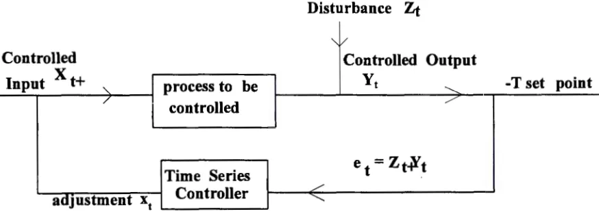
9 EXPRESSION FOR THE CONTROL ADJUSTMENT IN THE INPUT VARIABLE

OF A TIME SERIES CONTROLLER

An expression is derived for the feedback control adjustment required in the input

manipulated variable of a time series controller for a dynamic process with dead time (delay). This

the feedback control scheme to compensate a disturbance Zt by means of a time series controller.

Baxley [1991] considered the dead time equal to one period when deriving the feedback control

equation. In this Section, the feedback control (adjustment) algorithm is derived considering b

periods of deadtime. It is shown that it conforms to the minimum variance (mean square error)

control equation derived by Kramer [1990] for a system in which adjustments to the input variable

are made after the process is observed and so their effects are first seen at the next observation (b= 0).

Disturbance

Zt

'-,/

Controlled Controlled Output

x

Input t+

"

/

controlled /

et= Zt.¥t Time Series

I

Controller / adjustment xt I ...

Figure 4 Feedback Control scheme to compensate disturbance Zt

in a Time Series Controller . in the existence of Dynamics and Deadtime

From (5),

-T set point

Changes are made in the controlled input X at times t,t-l ,t-2,---, immediately after

observing the disturbances zt,zt-1,zt-2,---.

Because of this, a pulsed input results and the level of X in the interval t to t+ 1 is denoted by Xt+

For this pulsed input, assume that the dynamic model which connects the input manipulated

variable Xt+ and the controlled output Y t is

y t=L 1-1 (B)L2(B )B b+ 1 Xt+'

where,

Li (B) is a polynomial in B of degree r,

L1(B) is a polynomial in B of degree s and

b is the number of complete intervals of pure delay before an adjustment in the input Xt+ begins to

affect the output Y t·

The nonstationary disturbance is represented by the ARIMA (0, 1, 1) model

VZt

Zt measures the effect at the output of an unobserved disturbance, that is, an uncompensated

nonstationary disturbance that reaches the output before it is possible for the compensating control

action to become effective, this causes the process to wander off target. It is defined as the deviation

from the target that would occur if no control action was taken. The effect of the disturbance would

be cancelled if it was possible to set

Xt+ = -L1 (B)L2-1(B)Zt+b+1

This control action is not realisable since (b+ 1) is positive; but, the minimum mean square error of

the deviation of the output from its target value can be obtained by replacing Zt+b+ 1 by its forecast

A

estimate Zt(b+ 1) made at time t.

That is, by taking the minimum variance control action

A

(7)

The change or adjustment to be made in the input manipulated variable is then

A /\

(8)

The error at the output or deviation from the target at time (t+b+ 1) is the forecast error et(b+ 1) at

lead time b+ 1 for the Zt disturbance.

That is,

made (b+ 1) steps ahead at time t.

The error observed at time t is

Et= et-b -1 (b+l)

"

" "

Zt(b+ 1) -Zt-1(b+1) can be deduced from the observed error sequence Et,_{Et- l ,Et_2,-}--.

"

~ (b+l) and Zt(b+l) are linear functions of the {~}'s.

So,

Zt+b+l = L4(B)~+b+l + L3(B)~ where '

L3(B) and L4(B) are operators in B which can be deduced from the relations

From these,

"

and

"

Zt(b+l) = {1- 0/ 1-B}~ = L3(B)~, giving L3(B) = 1-011-B.

Similarly, L4(B) is found by expressing the forecast errors as a linear function of future shocks (Box

and Jenkins [page 128, 1970,1976]).

Then,

Ll(B) = (1- 01B - 02B2),

L1(B) = PG(l- 01 - 02)

L3(B) = (1-0)/(1-B) and

So, for a time series controller, when the disturbance is described by the ARIMA (0, I, I) model and

there are definite carry over effects, the· adjustment (xt) in the input manipulated variable required to

make the control and forecast error variances equal, is given by

(Box and Jenkins [1970,1976])

The control action in terms of the adjustment x

=

t t+ t-1+

- LI (B) L3(B)(l - B) Xt = L2(B)14 (B) Et

(equation 12.2.8 page 435 Box and Jenkins [1970,1976]).

This 'feedback control equation defines the adjustment to be made to the process at time t

which would produce the feedback control action yielding the smallest possible mean square error

since it exactly compensates the predicted deviation from target' (page 213, Box and Jenkins

[1968b]).

The above equation, on substituting the_ expressions for L1 (B), L2(B), L3(B) and L4(B), results in

(I- 01B-02 B2)(1-0)

Xt = - Et

PG(l-01-02)(1 + (l-0)B) (9)

where 0 is the moving average (operator) parameter.

The control (forecast) errors which turn out to be the one-step ahead forecast errors are measured in

practice.

It is known that the forecast error Et at the output at time t is the forecast error at lead time b+ 1 for

the

Zt

So,

·

Et=

WI =1-0, so

= (1

+

and further,

( -01B-02B2)(1-0)

Xt = - 1 (1+(1-0)B) PG(l-01-02)(1+(1-0)B) at

Since (1 - 0) x 100 per cent of the control error will affect the future process behaviour as per the

disturbance model, for a dead time b,

and so

et=~+ (1-0)~-b

= ~[1

+

Therefore, the control adjustment equation for b periods of deadtime is

(l-01 B-02B2)(1-0) et

Xt

= -

---0---PG(l - 01 - 02) (1 + (1-0) Bb)

That is,

givmg

(11)

(12)

The control adjustment action given by (12) minimises the variance of the output controlled variable.

Equation (12) is in conformance with the feedback control action adjustment equation

of Kramer [1990] when the output variance is made equal to the variance (cra2) of the random

adjustment action is made up of the current deviation (et) and the past adjustment action xt-b

(Kramer [1990]). It is observed also that this is similar to the feedback control action adjustment

equation for one period of deadtime derived by Baxley [1991] on taking a value 1 for b, the deadtime

and when there are no carry-over effects for a 'standard' time series controller. On comparison with

the equation of Baxley [ 1991], it is found that the first term in equation 12 gives the integral action

and the second term, the deadtime compensator, developed by Smith [1959] (Baxley [1991]).

Some simulation results of equation 12 obtained when b = 1, (Table 1) match closely

with that ofBaxley's [1991] values for the time series controller.

10 CONCLUSION

This report, having discussed briefly the need for stochastic models has provided a brief

discussion of minimum variance control and time series controllers. A general feedback control

equation has been derived and a statistical control algorithm developed for the critically damped

REFERENCES

(I) Astrom, K.J. (1970). Introduction to Stochastic control theory.

Mathematics in Science and Engineering series, Volume 70, Academic Press, New

York.

(2) Barnard, G. A. (1959). Control Charts and Stochastic Processes,

Journal of the Royal Statistical Society, Series B, 21, 239-271.

(3) Bather, J. A. (1963). Control Charts and the Minimisation of Costs,

Journal of the Royal Statistical Society, Series B, 25, 49-80.

(4) Baxley, Robert V. (1991). A Simulation Study Of Statistical Process

Control Algorithms For Drifting Processes, SPC in Manufacturing,Marcel

Dekker,Inc., NewYork and Basel.

(5) Box, G.E.P. and Jenkins, G.M. (1963). Further Contributions To

Adaptiv Control: Simultaneous Estimation Of Dynamics: Non-Zero Costs,

Statistics in Physical Sciences I, 943-974.

(6) Box, G.E.P. and Jenkins, G.M. (1965). Mathematical models for

adaptive control and optimisation. A.I Chem.E. - Chem. E. Symposium Series, 4:

61-68.

(7) Box, G.E.P. and Jenkins, G.M. (1968). Some Recent Advances in

Forecasting and Control, Part I, Journal of Royal Statistical Society, Applied

Statistics, Series C, 91-109.

(8) Box, G.E.P. and Jenkins, G.M. (1970, 1976). Time Series Analysis:

(9) Box, G.E.P., Jenkins, G.M and MacGregor J.P., (1974). Some Recent

Advances in Forecasting and Control, Part II, Applied Statistics, 23, No. 2,

158-179.

(IO) Box, G.E.P. and Kramer, T. (1990). Statistical Process Control and

Automatic Process Control - A Discussion, technical report no. 41 of the Centre

for Quality and Productivity Improvement, University of Wisconsin, U.S.A.

(11) Box, G.E.P. and Kramer, T. (1992). Statistical Process Monitoring and

Feedback Adjustment--A Discussion, Technometrics, August 1992, Volume 34,

No. 3, 251-267.

(12) . Deshpande, P.B and Ash, R.H., (1981). Elements of Computer Process

Control with Advanced Control Applications, Instrument Society of America,

North Carolina, U.S.A.

(13) Hall, A.C., (1956). Frequency response, Macmillan, New York.

(14) Harris,T.J.,MacGregor,J.F. and Wright J.D. (1981). An overviewof

Discrete stochastic Controllers:Generalized PID Algorithms with Dead-Time

Compensation, Can. J. Chem. Eng. 60, 425-432.

(15) Harris,T.J. (1989). Interfaces between statistical process control and

engineering process control, University of Wisconsin.

(16) Keats, J.B.and Hubele, N.F., (1989). Statistical Process Control In

Automated Manufacturing, Marcel Dekker, Inc., New York and Basel.

(17) Kramer, T.(1990). Process control from an economic point of

view-Industrial process control, technical report no.42 of the Centre for Quality and

(18) Kramer, T, (1990). Process control from an economic point of view-Dynamic adjustment and quadratic costs, technical report no.44 of the centre for Quality and Productivity Improvement, University ofWisconsin, U.S.A.

(19) MacGregor, J.F., (1987). Interfaces between process control and on-line statistical process control, Computing and Systems Technology division Communications, 10 (no.2): 9-20.

(20) MacGregor, J.F., (1988). On-line statistical process control, Chemical Engineering Progress, 84, 21-31.

(21) Palmor Z.J. and Shinnar R., Design of Sampled Data Controllers,

(1979). Industrial and Engineering Chemistry Process Design Development, Vol.18, No. I, 8-30.