Randomized Quasi-Random Testing

(1)

Randomized Quasi-Random Testing

Huai Liu,

Member, IEEE,

and Tsong Yueh Chen,

Member, IEEE

Abstract—Random testing is a fundamental testing technique that can be used to generate test cases for both hardware and software

systems. Quasi-random testing was proposed as an enhancement to the cost-effectiveness of random testing: In addition to having similar computation overheads to random testing, it makes use of quasi-random sequences to generate low-discrepancy and

low-dispersion test cases that help deliver high failure-detection effectiveness. Currently, few algorithms exist to generate quasi-random sequences, and these are mostly deterministic, rather than random. A previous study of quasi-random testing has examined two methods for randomizing quasi-random sequences to improve their applicability in testing. However, these randomization methods still have shortcomings — one method does not introduce much randomness to the test cases, while the other does not support

incremental test case generation. In this paper, we present an innovative approach to incrementally randomizing quasi-random sequences. The test cases generated by this new approach show a high degree of randomness and evenness in distribution. We also conduct simulations and empirical studies to demonstrate the applicability and effectiveness of our approach in software testing.

Index Terms—Random testing, quasi-random testing, randomized quasi-random sequence, adaptive random testing, failure-detection

effectiveness, test case distribution.

F

1 INTRODUCTION

R

ANDOMtesting (RT) [1], [35] is a basic testing technique,

involving selection of test cases in a random manner from theinput domain (the set of all possible inputs). It has been extensively used in the testing of hardware [21] and software systems [34]. RT can automatically generate a large number of test cases at low cost, using little information of the system under test, and with little human bias. Fur-thermore, its “randomness” helps make it possible to reveal failures that cannot be detected by some systematic testing techniques (such as those based on code coverage [46], finite state machines [22], and model checking [8]). RT has been successfully used to detect failures for various systems, such as network protocols implementations [44], Windows NT programs [20], and embedded systems [40].

A number of researchers [2], [4], [19], [45] from different areas have independently conducted investigations into the behavior and patterns of software failures, and have re-ported the common observation thatfailure-causing inputs

(those inputs that can reveal software failures) are normally clustered into contiguousfailure regions. Given that failure regions are contiguous, non-failure regions should also be contiguous. Suppose that a test case t does not reveal a failure, then test cases that are spread further away from t may have a higher chance of being failure-causing than those close to it (t’s neighbors): An even spread of test cases can help to improve the failure-detection effectiveness of RT. A number of innovative methods have been proposed based on this intuition, such as adaptive random testing (ART) [14] and quasi-random testing (QRT) [12].

A preliminary version of this paper was presented at the 9th International Conference on Quality Software (QSIC 2009) [28].

• H. Liu is with the Australia-India Research Centre for Automation Software Engineering, RMIT University, Australia.

E-mail: [email protected]

• T. Y. Chen is with the Department of Computer Science and Software Engineering, Swinburne University of Technology, Australia.

E-mail: [email protected]

QRT makes use of quasi-random sequences to generate test cases. Due to the low discrepancy and low disper-sion offered by quasi-random sequences, QRT can achieve an even distribution of test cases, which helps deliver a higher effectiveness of failure detection than RT. How-ever, quasi-random sequences face some significant chal-lenges with respect to testing, including that only a limited number of distinct quasi-random sequences exist, and that they are generated by deterministic algorithms. In other words, quasi-random sequences are less “random” than random/pseudorandom sequences. These issues restrict the applicability of quasi-random sequences in testing. To ad-dress these problems, Chen and Merkel [12] have exam-ined two methods to randomize quasi-random sequences, namely Cranley-Patterson Rotation [16] and Owen’s Scram-bling [38]. However, these two methods also have shortcom-ings: The former does not introduce much randomness into the sequences; while the latter requires advance knowledge of the number of test cases to be generated, that is, it does not allow for an incremental generation of test cases.

In a preliminary study [28], we have proposed an innovative approach to incrementally randomizing quasi-random sequences. In this paper, we not only present a formal algorithm with a more detailed discussion of the ap-proach, named randomized quasi-random testing (RQRT), but also conduct experimental studies to comprehensively demonstrate its applicability and effectiveness. A larger scale of simulations have been applied to show the test case distribution and failure-detection effectiveness of RQRT un-der various situations. In addition, an empirical study has been conducted to further demonstrate the effectiveness of RQRT for real-life programs and various faults.

(2)

discuss the threats to validity of our study, and Section 7 summarizes the paper.

2 BACKGROUND

2.1 Adaptive random testing

Failure-causing inputs decide two basic features of all faulty programs, thefailure rateand thefailure pattern. The failure rate (denotedθin this paper) refers to the ratio of the num-ber of failure-causing inputs to the numnum-ber of all possible inputs; the failure pattern refers to the geometry of failure regions, and their distributions over the input domain. The failure pattern has been investigated in various areas of soft-ware engineering, and it has been commonly observed that failure-causing inputs tend to cluster into contiguous failure regions [2], [4], [19], [45]. Based on such an observation, Chen et al. [14] proposed that test cases should be evenly spread over the input domain for achieving a high failure-detection effectiveness.

One popular approach to evenly spreading test cases is adaptive random testing (ART) [14]. There are various ART algorithms to achieve the notion of an even spread [14], [32], [41], [43], with a typical one being the fixed-size-candidate-set ART (FSCS-ART) [14]. FSCS-ART maintains two fixed-size-candidate-sets of test cases: the executed set (consisting of the executed test cases); and the candidate set (containing k randomly generated inputs as candidates for the next test case). A candidate is selected as the next test case if it has the greatest distance to its nearest neighbor in the executed set.

Many simulations and empirical studies have been con-ducted to examine the performance of ART, with its failure-detection effectiveness often evaluated and compared with that of RT, based on the F-measure, the expected number of test cases required to detect the first software failure. It has been shown that ART normally has a lower F-measure than RT, that is, ART normally requires fewer test cases to detect the first failure. In some circumstances, the F-measure of ART can be as low as 50% of that of RT, which is the theoretical upper bound for the effectiveness of a testing method [13].

2.2 Quasi-random sequences

Discrepancy and dispersion are two popular metrics for measuring how evenly a set of sample points are distributed inside ad-dimensional unit hypercubeId= [0,1)d.

Discrep-ancy examines whether different subdomains inIdhave an

equal density of points, and can be calculated [5], [7] as follows:

discrepancy = sup

D

A(D)

N −

|D| |Id|

, (1)

where N is the total number of sample points,D refers to any subdomain ofId,A(D)denotes the number of points

insideD,|·|is the size of a region/set, and suprepresents the supremum of a data set.

Dispersion measures the distribution by examining the size of the largest empty spherical region (containing no point) inside Id. One straightforward way to calculate

dis-persion is to measure the maximum distance from any point to its nearest neighbor [5].

Based on the definitions, we can say that lower discrep-ancy and dispersion indicate a more even distribution of the points.

Quasi-random sequences (point sequences with low dis-crepancy and low dispersion) are widely used in various do-mains, including global optimization [36], high-dimension integral approximation [24], and path planning [5]. Several algorithms [7], [26], [42] have been developed to generate different quasi-random sequences. The Sobol sequence [6], [42] is a popular quasi-random sequence, which can achieve a discrepancy of as low as O(logd_N_{). A Sobol sequence}

can be represented by a set of points T1, T2,· · ·, where

Ti = (t1i, t 2 i,· · ·, t

d

i) is the ith point in a d-dimensional

sequence, tj_i = p/2q is the jth coordinate of Ti, q is a

positive integer satisfying 2q−1 _≤ _{i <} ₂q_{, and} _p _{is an}

odd integer in the range (0,2q₎

that is decided through a series of complex calculations. For example, in a one-dimensional unit hypercubeI1= [0,1), the Sobol sequence

is:0.5(that is, 1/21_),₀_.₂₅₍₁_/₂2_),₀_.₇₅₍₃_/₂2_),₀_.₃₇₅₍₃_/₂3_),

0.875 (7/23), 0.125 (1/23), 0.625 (5/23), · · ·. In this paper, unless otherwise specified, the Sobol sequence is used as the quasi-random sequence.

2.3 Quasi-random testing

A major disadvantage of ART is that it normally incurs a high computational overhead: FSCS-ART, for example, requires O(n2₎ _{time to generate} _n _{test cases. The}

compu-tation overhead for generating n quasi-random points, in contrast, is only O(n), similar to that of pure RT. Chen and Merkel [12] proposed quasi-random testing (QRT), which applies quasi-random sequences in software testing. As discussed in Section 2.2, quasi-random sequences are generated using deterministic algorithms, and thus may not be as “random” as random/pseudorandom sequences. Chen and Merkel used two methods to randomize quasi-random sequences before applying them to test real-life pro-grams: Cranley-Patterson rotation [16] and Owen’s Scram-bling [38]. Cranley-Patterson rotation involves rotation of a quasi-random sequence using a random vector V = (v1_{, v}2_,_{· · ·} _{, v}d₎

insideId, wherevj is thejth coordinate of

V, and0≤vj <1. Each pointTi= (t1i, t 2 i,· · ·, t

d

i)in the

se-quence is displaced to a new positionT_i0= (t0_i1, t_i02,· · · , t0_id),

where t0_ij = (

tj_i+vj _if_tj

i+vj<1,

tj_i+vj−1 iftj_i+vj≥1. Owen’s Scram-bling [38] effectively implements random permutations of each point in the sequence. Compared with Cranley-Patterson rotation, Owen’s Scrambling is more precise in terms of maintaining the essential features of quasi-random sequences, such as low discrepancy and low dispersion.

(3)

In the following section, we present a novel approach which not only enables incremental test case generation, but also adds a high degree of randomness to the test cases.

3 RANDOMIZED

QUASI-RANDOM

TESTING

Given a quasi-random sequence, our randomization ap-proach consists of two steps: random shaking and ran-dom rotation. Firstly, anon-uniform distributionis used to shake the coordinates of each individual point in the quasi-random sequence into a quasi-random number within a specific value range. Then, as with the Cranley-Patterson rotation method, a randomly generated vector is applied to displace all points. In this study, thecosine distribution [33] is used to illustrate our approach — a random variablexconforms to the cosine distribution if its probability density function, pdf(x), is as follows:

pdf(x) = 1 2πB

1 + cos

_x₋_A

B

, (2)

where A and B are two real numbers deciding the value range ofx.

From Eqn. (2), we can getx∈[A−πB, A+πB], that is, Ais the central location ofx’s value range, andB decides the scale of the value range.

Fig. 1 showspdf(x)withA= 0andB= 1.

f(x)

0 0.1 0.2 0.3 0.4

-4 -3 -2 -1 0 1 2 3 4

x

Fig. 1. Cosine distribution

In order to distinguish our approach from the orig-inal QRT, we name it randomized quasi-random testing

(RQRT), and outline its algorithm below. Compared with the Cranley-Patterson rotation method, RQRT adds additional randomness through the random shaking (Statements 8 to 10 in the algorithm). In order to retain a low discrepancy and a low dispersion, a specific kind of distribution (such as the cosine one in this study) should be used to ensure that points closer to the centre of the value range (that is, the original Sobol point t1

i, t2i,· · ·, tdi

) have a higher probability of being selected into the randomized sequence. Compared with Owen’s scrambling method, our approach does not need to know in advance how many points are required, and can therefore incrementally randomize quasi-random points. Furthermore, the approach makes use of a parameter α (Statement 1 in the algorithm), the different values of which can result in different types of sequences:

Intuitively speaking, a smallerαimplies that the resulting sequences will maintain most attributes of quasi-random sequences (such as low discrepancy and low dispersion), but are less “random”; a largerαindicates that the resulting sequences are more random, but may lose some character-istics of quasi-random sequences.

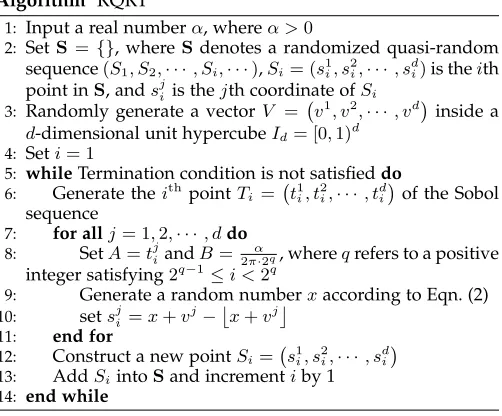
Algorithm RQRT

1: Input a real numberα, whereα >0

2: SetS={}, whereSdenotes a randomized quasi-random

sequence(S1, S2,· · ·, Si,· · ·),Si= (s1i, s2i,· · ·, sdi)is theith

point inS, andsj_i is thejth coordinate ofSi

3: Randomly generate a vectorV = v1, v2,· · ·, vd

inside a

d-dimensional unit hypercubeId= [0,1)d

4: Seti= 1

5: whileTermination condition is not satisfieddo

6: Generate theith _point_T

i= t1i, t2i,· · ·, tdi

of the Sobol sequence

7: for allj= 1,2,· · ·, ddo

8: SetA=tj_iandB= α

2π·2q, whereqrefers to a positive

integer satisfying2q−1_≤_{i <}₂q

9: Generate a random numberxaccording to Eqn. (2)

10: setsji=x+v

j₋

x+vj

11: end for

12: Construct a new pointSi= s1i, s2i,· · ·, sdi

13: AddSiintoSand incrementiby 1

14: end while

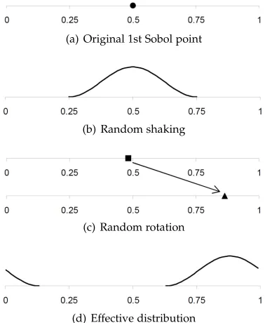
Figs. 2 and 3 further illustrate how RQRT randomizes the Sobol sequence when d = 1. As mentioned above, the randomization effectively consists of two steps: ran-dom shaking and ranran-dom rotation. After the original Sobol points are generated (refer to the circle dots in Figs. 2(a) and 3(a)), the cosine distribution is used to randomly shake the points (refer to the curves in Figs. 2(b) and 3(b)). Note that the range of the cosine distribution is dynamically adjusted throughout the testing process, as shown by the difference between the curves in Figs. 2(b) and 3(b). A pre-defined random vector is then used to further rotate the shaken points (refer to the square and triangle dots in Figs. 2(c) and 3(c)). Such a randomization process can also be regarded as random generation based on certain types of distributions, as shown in Figs. 2(d) and 3(d): RQRT generates test cases according to a dynamic profile, which is adjusted while test cases are incrementally generated.

4 EXPERIMENTAL

STUDIES

We conducted simulations and empirical studies to investi-gate the performance of RQRT. The design and settings of these experimental studies are discussed in this section.

4.1 Research questions

The main purpose of RQRT is to deliver high failure-detection effectiveness through an even spread of test cases. Our experimental studies aimed at answering the following two research questions:

RQ1 How evenly can RQRT distribute test cases? RQ2 How effectively can RQRT detect software

(4)

(a) Original 1st Sobol point

(b) Random shaking

(c) Random rotation

(d) Effective distribution

Fig. 2. Randomization of the 1st Sobol point

(a) Original 2nd and 3rd Sobol points

(b) Random shaking

(c) Random rotation

(d) Effective distribution

Fig. 3. Randomization of the 2nd and 3rd Sobol points

4.2 Variables and measures

4.2.1 Independent variables

The independent variable in our experiment is the test case selection strategy under study. Our proposed RQRT method is an obvious candidate. In addition, we selected three benchmark techniques to provide baselines for comparison. The first benchmark technique is RT. In reality, it is not easy to generate genuinely random inputs, especially according to a certain probability distribution. One popular way is to make use of pseudorandom number generators, which are widely used in various domains, such as com-puter modeling, and experiment design. In this study, we implemented RT based on the Mersenne Twister [31], which

can generate a large amount of pseudorandom numbers according to the uniform distribution.

ART was also selected as a benchmark technique because QRT (and RQRT) was motivated by the same fundamental principles as ART (that even spreading of test cases will enhance the failure-finding effectiveness). Among all ART algorithms, FSCS-ART was the first, and also the most studied one. For ease of comparison with the numerous previous studies on ART [9], [12], [30], we selected FSCS-ART as the FSCS-ART algorithm in our experiment. In the rest of this paper, unless otherwise specified, it is FSCS-ART being referred to when ART is mentioned.

RQRT is directly related to QRT, so it is important to include also QRT in our experiment. As mentioned above, QRT with Owen’s Scrambling does not support incremental generation of test cases — the number of test cases to be generated needs to specified in advance. Such a shortcoming is especially problematic for random techniques, such as RT, ART, QRT, and RQRT. The randomness in these tech-niques makes it extremely difficult to predict how many test cases would be required, even if testers have some prior knowledge of the failure rate. As shown in the previous study [11], the number of test cases to detect the first failure in each individual testing run (which, different from the F-measure, is defined as the F-count [13]) of RT or ART has a very large value range; for example, for a given failure rate θ, the F-count of RT will range from 1 to over 10/θ, even though the theoretical F-measure of RT is only 1/θ. The safest way to implement QRT with Owen’s Scrambling is to predefine a very large number for test case generation, but this may result in many generated test cases not being executed, and thus significantly reduce the efficiency and the cost-effectiveness of QRT, which is contrary to the ex-pected benefits of QRT. Because of this, we did not select QRT with Owen’s Scrambling as a benchmark technique, but instead chose QRT with Cranley-Patterson Rotation, which can generate test cases incrementally. In the rest of this paper, unless otherwise specified, QRT with Cranley-Patterson Rotation is intended when QRT is referred to.

A new ART method, random border centroidal voronoi tessellations (RBCVT), has recently been proposed [41], a search algorithm based on which (RBCVT-Fast) can achieve a similar computational overhead to QRT and RQRT. How-ever, because RBCVT-Fast faces the same challenge as QRT with Owen’s Scrambling, of not being able to generate test cases in a fully incremental way, it was also not selected as a benchmark technique in our study.

4.2.2 Dependent variables

For RQ1, we used the discrepancy and dispersion metrics to evaluate the test case distribution of RQRT. Because it would be extremely difficult, if not impossible, to obtain the exact value of discrepancy according to Eqn. (1), we calculated the approximate value as follows:

discrepancy≈max1000

i=1

A(Di)

N −

|Di|

|Id|

, (3)

whereN is the total number of test cases selected so far,Di

denotes a randomly selected subdomain of Id, and A(Di)

(5)

widely used in previous studies [9], [30] to approximate the value of discrepancy.

As explained in Section 2.2, the dispersion can be calcu-lated as the maximum distance from any point to its nearest neighbor, as shown in the following:

dispersion =max|S|

i=1 dist(Si, η(Si,S\Si)), (4)

wheredist(a, b)denotes the distance between two pointsa andb, andη(a,P)refers to pointa’s nearest neighbor in a set of pointsP.

For RQ2, similar to previous studies on ART and QRT [9], [12], [25], [30], [32], we evaluated the failure-detection effectiveness based on the F-measure, which refers to the expected number of test cases required to detect the first software failure, as defined in Section 2.1. Chen and Merkel [13] have demonstrated that the F-measure is particularly suitable for analyzing the effectiveness of random testing strategies (such as ART and RT), which normally generate test cases in an incremental way. The actual F-measure values depend not only on the individual testing technique, but also on the failure rates and failure patterns; furthermore, they do not conform to a normal distribution. To clearly and precisely show the differences in failure-detection effectiveness among the techniques under study, we therefore also used the F-ratio, which refers to the ratio between the F-measure of the testing technique under study (ART, RQRT, or QRT) and that of RT. Note that in the comparison among different techniques, the ranking of performance is the same for both the ratio and the F-measure.

4.3 Simulations

Chen and Merkel [12] conducted some simulations to derive the F-measure of the original QRT. However, these simu-lations were limited to the simple situation of there being only one single compact failure region (the most favorable condition for ART and QRT). Furthermore, although it is intuitive that RQRT or QRT should offer an even spread of test cases, few simulations [28] have been conducted to experimentally confirm the test case distribution. In this study, we have conducted more comprehensive simulations, through which we not only measure how evenly RQRT can spread test cases (for RQ1), but also evaluate its failure-detection effectiveness under various conditions (for RQ2).

In the simulations for RQ1, the input domain was de-fined as ad-dimensional unit hypercubeId = [0,1)d,d= 1,

2,3,4, and the number of test cases was set as100,500, 1000,1500,2000,· · ·,10000.

For RQ2, we evaluated the F-measures using simulations with similar experimental settings to those used in previous studies [9], [25], [30]. In these simulations, ad-dimensional unit hypercubeId was used to simulate the program input

domain. In order to simulate faulty programs, the failure rate (θ) and failure pattern were pre-defined, and the result-ing failure regions (whose size and shape were decided byθ and the failure pattern, respectively) were randomly placed inside the input domain. In our experiments, various failure patterns were used to show the relationship between the failure-detection effectiveness of RQRT and different factors. The simulated failure patterns are described as follows:

• In the first series of simulations, the failure pattern was defined as a single hypercube failure region, ran-domly placed withinId;dwas set to1,2,3,4,7, and

10; andθ was set to0.75,0.5,0.25,0.1,0.075,0.05, 0.025, 0.01, 0.0075, 0.005, 0.0025, 0.001, 0.00075, 0.0005,0.00025,0.0001,0.000075, and0.00005. The main purpose of these simulations was to examine to what extent the failure-detection effectiveness de-pends ondandθ.

• The second series of simulations examined the failure-detection effectiveness of RQRT on less com-pact failure regions. In these simulations,d = 2,3; θ = 0.001; and the failure pattern was defined as a single hyperrectangle failure region randomly placed within Id. For the hyperrectangle failure region, an

integral parameter γ was used to define the ratio among edge lengths of the rectangular/cuboid re-gions (1 :γ whend= 2and1 :γ :γ whend= 3). In our simulations,γwas set as1,4,7,10,20,30,40, 50,60,70,80,90, and 100. Note that γ = 1means the failure region is a hypercube. A hyperrectangle is less compact than a hypercube, with the compactness decreasing asγincreases.

• The objective of the third series of simulations was to investigate the performance of RQRT when there are multiple distinct failure regions. In these simulations, d = 2, 3; θ = 0.001; and the failure pattern was defined as a number (δ) of equal-sized hypercube failure regions randomly placed within Id, where

δ = 1, 4, 7, 10, 20, 30,40, 50, 60, 70, 80, 90, and 100.

• The fourth series of simulations were conducted to investigate the performance of RQRT when one failure region is predominant in size among all the distinct failure regions. In these simulations,d = 2, 3;θ= 0.001; andδ= 1,4,7,10,20,30,40,50,60,70, 80,90, and100. The failure pattern was defined asδ hypercube failure regions, with one region’s size set as 30%, 50%, or 80% of the total size for allδregions, and the remaining(δ−1)regions each being an equal proportion of the remaining size (70%, 50%, or 20%).

• In many practical situations, failure may not be re-lated to all input parameters. In the original ART algorithms, test cases are evenly spread in the d -dimensional input domain, but this may not guar-antee that they are also evenly distributed in any d0-dimensional space, where d0 < d: ART may not perform very well when the software fault is only related to some of the input domain parameters, as shown in previous studies [25]. In this study, we also conducted simulations to see whether such a problem can be solved by RQRT. In the simulations,θ was set to0.01,0.005,0.001, and0.0005; and the pair ofdand d0, denoted(d, d0), was set to (2,1),(3,1), (3,2),(4,1),(4,2), and(4,3). The failure pattern was defined as a single hypercube failure region in thed0 -dimensional space.

(6)

TABLE 1

Basic information of object programs

Program Basic function _d Input domain

From To

bessj0 Bessel function of the first kind 1 (−500) (500) bessj Bessel function of general integer order 2 (2,−500) (102,500)

plgndr Legendre polynomials associated with 3 (−1,10−1.1) (12,100,1.1)

spherical harmonics

select Select themth smallest element from 4 (−500,−500,−500,−500) (500,500,500,500)

an array containingnreal numbers∗

∗_{Note: In this study, we set}_n_{= 4}_and_m_{= 2}_{for the program}_select_{, that is,}_d_{= 4}_for_select_{in our experiment.}

a full picture of their performance. As shown in previous studies [9], [25], [30], ART has the best performance whenθ anddare small, and there is only one single compact failure region. However, the F-measure of ART becomes larger as d, θ, γ, and δ increase; furthermore, the failure-detection effectiveness of ART is similar to that of RT when the failure region is only present ind0-dimensional space (d0< d).

4.4 Object programs and mutants

Although simulations (reported in the previous section) can help provide a comprehensive picture of RQRT’s perfor-mance under various conditions (different failure patterns, θ,d, etc.), it is still necessary to conduct empirical studies to investigate its failure-detection effectiveness for real-life programs.

When choosing the object programs, one critical con-sideration was that they should accept numeric inputs — the application of quasi-random sequences to non-numeric program inputs, which is also a very challenging research project, is still under investigation. It was also necessary to consider that various factors should be involved in the empirical studies. Although it is often difficult to control the values of θand the failure patterns in empirical studies of real-life programs, it was still possible to choose programs with different values ofd(the number of input parameters of the program under test). In this study, four C programs (bessj0, bessj, pldndr, and select) were chosen as the object programs. These programs, which were extracted from Numerical Recipes [39], implement scientific functions, as summarized in Table 1. Among these programs,bessj0, bessj, andplgndrhave a fixed number of input parame-ters (d= 1,2, and3, respectively), and the programselect picks themth smallest element fromnreal numbers, where both m and n are changeable. Our investigation showed that different values ofmandnresulted in quite different features (including θ and failure patterns) in the mutant programs (the faulty versions created by seeding errors; to be discussed below). To better control the experiment, we fixed the values of m and n, setting n = 4 and m = 2, so that: (i) the programselect hasd = 4(different from the other three programs); and (ii) the program would not execute a simple function selecting the minimum (where m = 1) or maximum (wherem = 4) value, in which case a large portion of the program would not be executed or covered by most test cases.

Faults were seeded into the object programs based on the mutation analysis technique [17]. A C mutation tool,

Csaw [18], was used to generate various mutants, each of

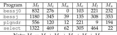
which was related to a single fault injected into an object program. Table 2 summarizes the statistical data for the mutants of each object program. In Table 2,Mtrefers to the

total number of mutants generated for each object program; Mi denotes the number of mutants that are syntactically

incorrect and thus cannot be compiled; Ma is the number

of mutants with execution problems (such as overflow and infinite loop);Merefers to the number of equivalent mutants

(that is, those mutants with θ = 0); Ml represents the

number of mutants with θ ≥ 0.1; and Ms denotes the

number of mutants with 0 < θ < 0.1. Readers can refer to a previous study [29] for how to distinguish different groups of mutants, such as the identification of equivalent mutants (related to Me), and the calculation of θ for each

mutant (related toMlandMs). In our study, we only used

the mutants with 0 < θ < 0.1, that is, the mutant sample size for each object program is actuallyMsin Table 2.

TABLE 2

Basic information of mutants

Program Mt Mi Ma Me Ml Ms

bessj0 832 276 0 103 221 232

bessj 1180 345 39 135 308 353

plgndr 556 120 12 221 9 194

select 1322 469 62 305 464 22

Note:Mt=Mi+Ma+Me+Ml+Ms.

4.5 Experiment design and data collection

4.5.1 Settings for RQRT

In the experiment, the cosine distribution (refer to Fig. 2) was used in the random shaking process of RQRT. The cosine distribution can be easily constructed by applying a basic function (cos−1₍_·_{)) to a uniformly distributed}

ran-dom variable. Although there are many other non-uniform distributions that have similar functions, their construction may involve more work — the triangle distribution, for example, requires two independent uniformly distributed random variables, and it would therefore be more expensive to implement this, or other complicated distributions (such as the semicircle).

To investigate the impact of different values of α, we selected RQRT withα= 0.1,1.0, and2.0, which are denoted by RQRT 0.1, RQRT 1.0, and RQRT 2.0, respectively.

4.5.2 Number of candidates in ART

(7)

candidate set (normally denoted by k) is determined by testers. Previous studies [14] have shown that the failure-detection effectiveness of ART improves as k increases, but becomes marginal after k exceeds 10. In line with the previous studies, in this study, we also setk= 10.

4.5.3 Discrepancy and dispersion

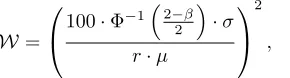
A sufficient amount (W) of data was collected to enable a reliable estimate of the mean value of discrepancy or dispersion, with a confidence level (1−β)×100%, and accuracy range±r%. Based on the central limit theorem, we can calculate

W= 



100·Φ−12−β 2

·σ

r·µ





2

, (5)

where µ and σ are the mean and the standard deviation of the metric, respectively; andΦ−1₍_·₎_{refers to the inverse}

standard normal distribution function. In our study, we set the confidence level to 95% (β = 0.05), and the accuracy range to±5%(r= 5).

4.5.4 F-measure

In the simulations, when a point inside a failure region was selected, a failure was said to be detected. In the empirical studies, a failure was detected in a mutant when a test case caused the mutant to show behavior different from that of the base program. In both the simulations and the empirical studies, test cases were generated until a failure was detected, with the number of test cases executed that far, the F-count (as defined in Section 4.2.1), recorded. Such a process was repeated until the mean F-count value could be considered as a reliable approximation of the F-measure with a 95% confidence level, and±5% accuracy range (refer to Eqn. (5) and the related discussion).

5 EXPERIMENTAL

RESULTS

5.1 Answer to RQ1: Test case distribution

The discrepancy and dispersion values for RQRT 0.1, RQRT 1.0, and RQRT 2.0 are given in Figs. 4 and 5, which, for ease of comparison, also include the results for RT, ART, and QRT.

From Figs. 4 and 5, it can be observed that the discrep-ancy values for the RQRT methods are significantly lower than those for ART and RT. With respect to dispersion, RQRT and ART have similar values, both being much lower than that of RT. Compared with QRT, RQRT has marginally higher discrepancy and dispersion, and, as expected, these values increase slightly as α increases. From these obser-vations, it can be concluded that the randomized quasi-random sequences generated by our approach still preserve a low discrepancy and a low dispersion: Overall, RQRT delivers a more even distribution of test cases than ART and RT.

5.2 Answer to RQ2 – Part 1: Failure-detection

effective-ness for various simulated failure patterns

5.2.1 Failudetection effectiveness for compact failure re-gions

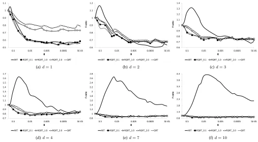
Fig. 6 shows the F-ratios of RQRT 0.1, RQRT 1.0, RQRT 2.0, ART and QRT for a single hypercube failure region.

Based on the simulations’ results, we can make the following observations:

• All three RQRT methods always have F-ratios less

than1, that is, RQRT always outperforms RT in terms of the F-measure.

• Among the three RQRT methods, RQRT 0.1 has the best performance, followed by RQRT 1.0, and then RQRT 2.0. In other words, the failure-detection ef-fectiveness of RQRT improves asαdecreases.

• Whendandθ are small, ART performs better than

RQRT, but when dor θ is large, RQRT can outper-form ART.

• QRT outperforms RQRT whend= 1, but they have

similar effectiveness whend >1.

The results, in terms of the performance ranking among QRT and the three RQRT methods, are as expected, and mir-ror the ranking observed for discrepancies and dispersion (Figs. 4 and 5). The results also imply that, in addition to test case distribution (measured by discrepancy and dispersion in this study), there are other factors (such asdandθ) that are strongly correlated with the failure-detection effective-ness: In particular, ART may have worse performance than RT when θor dis very large, conditions which have been documented as unfavorable for ART [9], [30]. In contrast, the impact ofdandθon RQRT’s performance is less significant: Although F-measure values for RQRT also increase asdor θincreases, the change is much less than that for ART.

5.2.2 Relationship between failure-detection effectiveness and failure region compactness

Fig. 7 shows the failure-detection effectiveness for a single hyperrectangle failure region, with various values ofγ.

From Fig. 7, it can be observed that, unlike ART (whose performance deteriorates with less compact failure regions), RQRT performs consistently well, regardless of the failure region compactness. RQRT and QRT have similar perfor-mance for this kind of failure pattern.

5.2.3 Relationship between failure-detection effectiveness and the number of distinct failure regions

Fig. 8 reports the failure-detection effectiveness for multiple equal-sized hypercube failure regions, with various values ofδ.

(8)

0.00 0.02 0.04 0.06 0.08 0.10 0.12

0 2000 4000 6000 8000 10000

D is cr e p a n cy

Number of test cases

RT ART RQRT_0.1 RQRT_1.0 RQRT_2.0 QRT

(a)d= 1

0.00 0.02 0.04 0.06 0.08 0.10 0.12

0 2000 4000 6000 8000 10000

D is cr e p a n cy

(b)d= 2

0.00 0.01 0.02 0.03 0.04 0.05 0.06 0.07 0.08 0.09 0.10

0 2000 4000 6000 8000 10000

D is cr e p a n cy

(c)d= 3

0.00 0.01 0.02 0.03 0.04 0.05 0.06 0.07 0.08

0 2000 4000 6000 8000 10000

D is cr e p a n cy

(d)d= 4

Fig. 4. Discrepancy of various methods

0.00 0.01 0.02 0.03

0 2000 4000 6000 8000 10000

D is p e rs io n

(a)d= 1

0.00 0.02 0.04 0.06 0.08 0.10 0.12 0.14 0.16

0 2000 4000 6000 8000 10000

D is p e rs io n

(b)d= 2

0.05 0.10 0.15 0.20 0.25 0.30

0 2000 4000 6000 8000 10000

D is p e rs io n

(c)d= 3

0.10 0.15 0.20 0.25 0.30 0.35 0.40 0.45

0 2000 4000 6000 8000 10000

D is p e rs io n

(d)d= 4

Fig. 5. Dispersion of various methods

5.2.4 Relationship between failure-detection effectiveness and predominant failure region size

Fig. 9 shows the failure-detection effectiveness for multiple hypercube failure regions with one predominant region.

Based on Fig. 9, it can be observed that when there is a predominant failure region, RQRT has a similar perfor-mance to ART and QRT; that all techniques outperform RT; and that their performance improves as the relative size of the predominant region increases.

5.2.5 Failure-detection effectiveness when the failure is not related to all input parameters

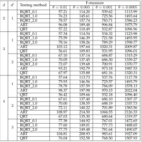
Table 3 summarizes the F-measures for RQRT when only some input parameters are failure-related.

It can be observed from Table 3 that, unlike ART, RQRT (and QRT) continues to have lower F-measures than RT when the software failure is only related to some of the input parameters (d0 < d). This result is actually not sur-prising, because a theoretical foundation for quasi-random sequences includes that if the sequence has low discrepancy and low dispersion in Id, then it will also have low

dis-crepancy and low dispersion in any d0-dimensional space (d0< d) [37].

In summary, as guaranteed with an even spread of test cases in anyd0-dimensional space, RQRT constantly delivers a better performance than RT, regardless of whether the failure is related to all or only some of the input parameters.

5.3 Answer to RQ2 – Part 2: Failure-detection

effective-ness for object programs

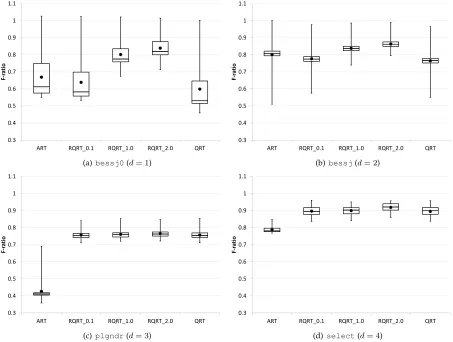
The results of the empirical studies for each object program are summarized in Fig. 10. In the figure, the boxplot displays the range of F-ratios for each of the three RQRT methods, for ART, and for QRT, with the lower and upper bounds of the box denoting the 1st and 3rd quartiles of F-ratios,

respectively. The line inside the box indicates the median F-ratio; the bottom and top whiskers represent the minimum and maximum F-ratio values, respectively; and the dot denotes the average F-ratio across all mutants under study for each object program.

Based on Fig. 10, the following observations can be made:

• For the overwhelming majority of mutants, all three RQRT methods have F-ratios less than1, that is, their F-measures are generally less than those of RT.

• RQRT 0.1 outperforms ART forbessj0andbessj, but not for plgndr or select. ART outperforms RQRT 1.0 and RQRT 2.0 for all object programs.

• The average F-ratio values for QRT are always less than those for RQRT.

• RQRT 0.1 always has better performance than

RQRT 1.0 and RQRT 2.0 in terms of F-measures.

The first observation is as expected: By making use of low-discrepancy and low-dispersion sequences, RQRT achieves a better failure-detection effectiveness than RT.

Although the second observation is not very consistent with the simulation results, it should be noted that no mat-ter how many real-life programs are examined, empirical studies can only represent some special cases, and may especially favor a particular technique. In this study, the performance of ART withplgndrwas very good. A further investigation determined that the plgndr mutants have low θ values (between 0.00012 and 0.00258), a condition known to be favorable for ART [9], [30], and therefore explaining ART’s good performance.

(9)

0.5 0.6 0.7 0.8 0.9 1 1.1 5E-05 0.0005 0.005 0.05 0.5 F -r a t io θθθθ

ART RQRT_0.1 RQRT_1.0 RQRT_2.0 QRT

(a)d= 1

0.6 0.7 0.8 0.9 1 1.1 1.2 5E-05 0.0005 0.005 0.05 0.5 F -r a t io θθθθ

(b)d= 2

0.6 0.7 0.8 0.9 1 1.1 1.2 1.3 1.4 5E-05 0.0005 0.005 0.05 0.5 F -r a t io θθθθ

(c)d= 3

0.7 0.8 0.9 1 1.1 1.2 1.3 1.4 1.5 1.6 1.7 5E-05 0.0005 0.005 0.05 0.5 F -r a t io θθθθ

(d)d= 4

0.8 1 1.2 1.4 1.6 1.8 2 2.2 2.4 2.6 2.8 5E-05 0.0005 0.005 0.05 0.5 F -r a t io θθθθ

(e)d= 7

0.8 1.3 1.8 2.3 2.8 3.3 3.8 4.3 5E-05 0.0005 0.005 0.05 0.5 F -r a t io θθθθ

(f)d= 10

Fig. 6. Failure-detection effectiveness of various methods for a single hypercube failure region

0.6 0.7 0.8 0.9 1 1.1

0 10 20 30 40 50 60 70 80 90 100

F -r a t io γγγγ

(a)d= 2

0.6 0.7 0.8 0.9 1 1.1

0 10 20 30 40 50 60 70 80 90 100

F -r a t io γγγγ

(b)d= 3

Fig. 7. Failure-detection effectiveness of various methods for a single hyperrectangle failure region

0.6 0.7 0.8 0.9 1 1.1

0 10 20 30 40 50 60 70 80 90 100

F -r a t io δδδδ

(a)d= 2

0.6 0.7 0.8 0.9 1 1.1

0 10 20 30 40 50 60 70 80 90 100

F -r a t io δδδδ

(b)d= 3

(10)

0.6 0.7 0.8 0.9 1 1.1

0 10 20 30 40 50 60 70 80 90 100

F

-r

a

t

io

δδδδ

(a) 30% predominant,d= 2

0.6 0.7 0.8 0.9 1 1.1

0 10 20 30 40 50 60 70 80 90 100

F

-r

a

t

io

δδδδ

(b) 50% predominant,d= 2

0.6 0.7 0.8 0.9 1 1.1

0 10 20 30 40 50 60 70 80 90 100

F

-r

a

t

io

δδδδ

(c) 80% predominant,d= 2

0.6 0.7 0.8 0.9 1 1.1

0 10 20 30 40 50 60 70 80 90 100

F

-r

a

t

io

δδδδ

(d) 30% predominant,d= 3

0.6 0.7 0.8 0.9 1 1.1

0 10 20 30 40 50 60 70 80 90 100

F

-r

a

t

io

δδδδ

(e) 50% predominant,d= 3

0.6 0.7 0.8 0.9 1 1.1

0 10 20 30 40 50 60 70 80 90 100

F

-r

a

t

io

δδδδ

(f) 80% predominant,d= 3

Fig. 9. Failure-detection effectiveness of various methods with multiple hypercube failure regions with a predominant region

0.3 0.4 0.5 0.6 0.7 0.8 0.9 1 1.1

F

-r

a

t

io

(a)bessj0(d= 1)

0.3 0.4 0.5 0.6 0.7 0.8 0.9 1 1.1

F

-r

a

t

io

(b)bessj(d= 2)

0.3 0.4 0.5 0.6 0.7 0.8 0.9 1 1.1

F

-r

a

t

io

(c)plgndr(d= 3)

0.3 0.4 0.5 0.6 0.7 0.8 0.9 1 1.1

F

-r

a

t

io

(d)select(d= 4)

(11)

TABLE 3

F-measures of various methods when the failure is related to only some of the input parameters

d d0 _{Testing method} F-measure

θ= 0.01 θ= 0.005 θ= 0.001 θ= 0.0005

2 1

RQRT 0.1 57.21 114.20 539.62 1113.99

RQRT 1.0 76.23 145.61 725.56 1493.64

RQRT 2.0 78.57 157.74 783.71 1586.23

ART 96.08 189.48 996.84 1975.79

QRT 57.22 110.49 532.87 1096.96

3 1

RQRT 0.1 57.34 114.54 534.32 1123.98

RQRT 1.0 75.59 146.39 721.58 1493.95

RQRT 2.0 78.16 158.26 789.29 1598.77

ART 103.12 197.64 1020.31 2009.87

QRT 56.61 109.83 531.95 1096.01

2

RQRT 0.1 67.10 137.14 684.87 1315.29

RQRT 1.0 70.05 137.45 686.30 1339.27

RQRT 2.0 72.07 139.68 700.91 1370.77

ART 93.21 192.79 973.18 1987.53

QRT 67.97 135.88 681.16 1320.31

4 1

RQRT 0.1 57.64 113.73 537.76 1117.78

RQRT 1.0 75.93 146.56 725.57 1493.79

RQRT 2.0 78.78 157.59 784.09 1578.13

ART 98.37 197.98 970.15 2022.04

QRT 56.42 109.66 532.18 1096.40

2

RQRT 0.1 67.61 137.40 686.10 1307.37

RQRT 1.0 70.00 138.55 688.19 1337.73

RQRT 2.0 72.11 140.22 701.89 1383.56

ART 108.97 214.50 1044.55 2126.33

QRT 67.03 135.30 680.64 1319.57

3

RQRT 0.1 77.38 144.92 767.01 1472.65

RQRT 1.0 77.60 149.01 777.73 1488.65

RQRT 2.0 77.75 149.48 781.64 1490.07

ART 104.81 208.93 983.61 1927.09

QRT 76.04 152.58 768.50 1507.93

empirical studies, we can conclude that both QRT and RQRT outperform RT.

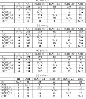
Table 4 summarizes a further comparison of the F-measures for all testing techniques applied to all mutants of the object programs. In the table, each cell contains the number of mutants for which the technique named in the topmost cell has better failure-detection effectiveness (a lower F-measure) than the technique named in the leftmost cell — for example, the number “353” in the top right cell in Table 4(b) means that QRT outperforms RT for all 353 mutants of bessj. Because the F-measures do not follow normal distribution, parametric hypothesis testing cannot be applied to analyze the results. In this study, therefore, hy-pothesis testing based on the Holm-Bonferroni method [23] was used to determine the statistical significance of the performance differences. In the hypothesis testing, there were totally 60 (= 4programs×15pairs of techniques) null hypotheses (H0), each of which was that each pair of testing

techniques have similar F-measures on a certain program. For each pair of technique on every object program, we calculated the p-value, and ordered all the 60 p-values from smallest to largest, that is, p1 ≤ p2 ≤ · · · ≤ p60. Given

the significance level 0.05, we found the minimal indexl such thatpl> ₆₁0.05₋_l. All the null hypotheses associated with

p1, p2, . . . , pl−1 were rejected, while other hypotheses were

not. Rejection of H0implies that the difference in F-measures

between the two techniques was statistically significant, a situation indicated byboldtypeface in Table 4.

The hypothesis testing results show that RQRT sig-nificantly outperforms RT in terms of F-measures. When comparing RQRT with ART, it was found that for two

ob-ject programs (bessj0andbessj), RQRT 0.1 significantly outperforms ART, but for other cases (RQRT 0.1 compared with ART for plgndr and select, and RQRT 1.0 and RQRT 2.0 compared with ART for all four programs), ART significantly outperforms RQRT; in other words, we cannot statistically distinguish the failure-detection effectiveness of RQRT and ART. Given that RQRT has a very low compu-tational overhead (O(n), the same as RT), RQRT is more cost-effective than RT and ART. The results show that, except in three cases (RQRT 0.1 compared with QRT for plgndr; and RQRT 0.1 compared with QRT, and RQRT 1.0 compared with QRT forselect), QRT significantly outper-forms RQRT.

(12)

TABLE 4

Pairwise comparison of F-measures among RT, ART, QRT, and RQRT

(a)bessj0

RT ART RQRT 0.1 RQRT 1.0 RQRT 2.0 QRT

RT N/A 228 231 229 230 231

ART 4 N/A 212 7 7 224

RQRT 0.1 1 20 N/A 7 5 220

RQRT 1.0 3 225 225 N/A 10 231

RQRT 2.0 2 225 227 222 N/A 231

QRT 1 8 12 1 1 N/A

(b)bessj

RT N/A 352 353 353 353 353

ART 1 N/A 317 11 1 331

RQRT 0.1 0 36 N/A 7 3 256

RQRT 1.0 0 342 346 N/A 17 346

RQRT 2.0 0 352 350 336 N/A 350

QRT 0 22 97 7 3 N/A

(c)plgndr

RT N/A 194 194 194 194 194

ART 0 N/A 0 0 0 0

RQRT 0.1 0 194 N/A 75 52 92

RQRT 1.0 0 194 119 N/A 69 113

RQRT 2.0 0 194 142 125 N/A 139

QRT 0 194 102 81 55 N/A

(d)select

RT N/A 22 22 22 22 22

ART 0 N/A 1 0 0 1

RQRT 0.1 0 21 N/A 11 2 12

RQRT 1.0 0 22 11 N/A 3 11

RQRT 2.0 0 22 20 19 N/A 17

QRT 0 21 10 11 5 N/A

the difference between QRT and RQRT: QRT has a more even test case distribution, but with less randomness. In summary, there is a trade-off in the test cases generated by RQRT methods between the even-spreading (which is strongly correlated with good failure-detection effective-ness) and the randomness (which is related to the stability of the effectiveness).

6 THREATS TO

VALIDITY

The threats to the validity of this study are discussed in this section.

The main potential threat to internal validity is related to the implementation of the RQRT methods, which, because of the availability of a popular Sobol sequence generator [7], only required a small amount of programming. All the code has been carefully checked, and we are confident that all the testing methods were correctly implemented in our experiments. One major drawback of our implementation is the dimensionality: The Sobol sequence generator we used can only generate Sobol sequences with the dimension from 1 to 40; thus, the RQRT methods under study in this paper cannot be applied to the programs with much higher dimensions. Nevertheless, there exist other quasi-random sequences and generators in the literature, and the application of them into RQRT will result in more RQRT implementations that can be used in higher dimensional cases.

The major threat to external validity concerns the set-tings in the experiments. Although a number of different conditions (failure patterns,θ,d, etc.) have been considered in the simulations, it is extremely difficult, if not impossible, to comprehensively imitate the real-life scenarios. Further-more, the object programs and fault-seeded mutants used in the empirical studies were just special cases, and cannot fully represent the general case. Even though we have conducted both simulations and empirical studies, it is not possible to claim that our conclusions are universally valid, for any program.

The threat to construct validity relates to the measure-ment: In this study, we used the F-measure to evaluate and compare the failure-detection effectiveness of RQRT, ART, QRT, and RT. As discussed in Section 2.1, the F-measure is particularly suitable for random testing strategies, which normally generate test cases in an incremental way. Com-pared with the F-measure, the other two popular measures (the P-measure – the probability of at least one failure being detected by a given set of test cases; and the E-measure – the expected number of failures to be detected by a given set of test cases) both require that the number of test cases be known in advance, and are thus less appropriate for measuring the effectiveness of a random testing strategy such as RQRT.

(13)

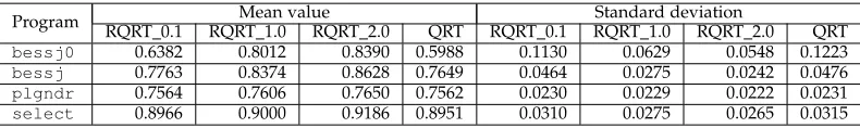
TABLE 5

Mean values and standard deviations of F-ratios for RQRT

Program Mean value Standard deviation

RQRT 0.1 RQRT 1.0 RQRT 2.0 QRT RQRT 0.1 RQRT 1.0 RQRT 2.0 QRT

bessj0 0.6382 0.8012 0.8390 0.5988 0.1130 0.0629 0.0548 0.1223

bessj 0.7763 0.8374 0.8628 0.7649 0.0464 0.0275 0.0242 0.0476

plgndr 0.7564 0.7606 0.7650 0.7562 0.0230 0.0229 0.0222 0.0231

select 0.8966 0.9000 0.9186 0.8951 0.0310 0.0275 0.0265 0.0315

sufficiently large number of experimental runs to guarantee statistically reliable F-measure values, and hypothesis test-ing was conducted to verify the statistical significance of the empirical study results.

7 CONCLUSION

The failure-detection effectiveness of random testing (RT) can be improved by evenly spreading the test cases across the input domain. Adaptive random testing (ART) is a fam-ily of algorithms that achieve this notion of an even spread. Many ART algorithms, however, have high computational overhead, which may reduce their cost-effectiveness in test-ing, and thus affect their use in practice. Quasi-random testing (QRT) was proposed as an enhancement to the failure-detection effectiveness of RT, while maintaining the computational overhead at linear order. In QRT, test cases are generated based on quasi-random sequences, which are sets of points with low discrepancy and low dispersion. However, the two randomization methods used in the original QRT have some shortcomings, including that one does not introduce much randomness into the sequences, and that the other does not support incremental test case generation.

In this paper, we have presented an innovative approach to randomizing quasi-random sequences using a simple non-uniform distribution. The approach, randomized QRT (RQRT), can produce many random sequences with low discrepancy and low dispersion, and normally performs significantly better than pure RT in terms of the F-measure — but maintains the same linear order of computational overhead as RT. Compared with ART, RQRT has a very low computational overhead, but, as shown in the experimental studies, has a comparable failure-detection effectiveness, meaning that RQRT is the more cost-effective technique. Compared with the original QRT, RQRT not only introduces more randomness to the test cases but also supports their incremental generation.

The most important future work relates to extension of RQRT into more complicated non-numeric application do-mains. Although the randomized quasi-random sequences are naturally applicable to programs with numeric inputs, it is critical, yet challenging, to expand the research into converting these pure numeric sequences into test cases of complex input types, a step which will significantly improve the applicability of RQRT. Since some research has already been conducted into applying ART to non-numeric domains [3], [15], [27], one potential research direction is to investigate how to integrate RQRT with these studies. In addition, because it has been demonstrated that ART can achieve higher code coverage than RT [10], RQRT should also be able to deliver high coverage, something which

should be evaluated using more empirical studies. In this paper, we have used only one simple non-uniform distribu-tion (the cosine distribudistribu-tion), to illustrate our randomizadistribu-tion approach, but many other non-uniform distributions have been identified in the literature that have similar attributes to this distribution: It will be worthwhile to study the applicability and effectiveness of different distributions in the randomization of various quasi-random sequences. It was also observed that there is a trade-off between the randomness and the even distribution, which will also be an interesting topic for further study.

ACKNOWLEDGMENT

The authors would like to thank Dave Towey for the invalu-able discussion.

REFERENCES

[1] V. D. Agrawal. When to use random testing. IEEE Transactions on

Computers, 27(11):1054–1055, 1978.

[2] P. E. Ammann and J. C. Knight. Data diversity: an approach to

software fault tolerance.IEEE Transactions on Computers, 37(4):418–

425, 1988.

[3] A. Barus, T. Y. Chen, F.-C. Kuo, H. Liu, R. Merkel, and G.

Rother-mel. A novel linear algorithm for adaptive random testing on programs with non-numeric inputs. Technical Report TR-UNL-CSE-2014-0004, University of Nebraska – Lincoln, 2014.

[4] P. G. Bishop. The variation of software survival times for different

operational input profiles. InProceedings of the 23rd International

Symposium on Fault-Tolerant Computing, pages 98–107, 1993.

[5] M. S. Branicky, S. M. LaValle, K. Olson, and L. Yang.

Quasi-randomized path planning. In Proceedings of the 2001 IEEE

In-ternational Conference on Robotics and Automation, pages 1481–1487, 2001.

[6] P. Bratley and B. Fox. Algorithm 659: Implementing sobol’s

quasir-andom sequence generator. ACM Transactions on Mathematical

Software, 14(1):88–100, 1988.

[7] P. Bratley and B. Fox. Implementation and tests of low discrepancy

sequences.ACM Transactions on Modeling and Computer Simulation,

2(3):195–213, 1992.

[8] M. Chen and P. Mishra. Property learning techniques for efficient

generation of directed tests. IEEE Transactions on Computers,

60(6):852–864, 2011.

[9] T. Y. Chen, F.-C. Kuo, and H. Liu. Application of a failure driven

test profile in random testing. IEEE Transactions on Reliability,

58(1):179–192, 2009.

[10] T. Y. Chen, F.-C. Kuo, H. Liu, and E. W. Wong. Code

cover-age of adaptive random testing. IEEE Transactions on Reliability,

62(1):226–237, 2013.

[11] T. Y. Chen, F.-C. Kuo, and R. Merkel. On the statistical properties of

testing effectiveness measures.The Journal of Systems and Software,

79(5):591–601, 2006.

[12] T. Y. Chen and R. Merkel. Quasi-random testing.IEEE Transactions

on Reliability, 56(3):562–568, 2007.

[13] T. Y. Chen and R. Merkel. An upper bound on software

test-ing effectiveness. ACM Transactions on Software Engineering and

Methodology, 17(3):16:1–16:27, 2008.

[14] T. Y. Chen, T. H. Tse, and Y. T. Yu. Proportional sampling strategy:

A compendium and some insights. The Journal of Systems and

(14)

[15] I. Ciupa, A. Leitner, M. Oriol, and B. Meyer. ARTOO: adaptive

random testing for object-oriented software. In Proceedings of

the 30th International Conference on Software Engineering (ICSE’08), pages 71–80. ACM Press, 2008.

[16] R. Cranley and T. N. L. Patterson. Randomization of number

theoretic methods for multiple integration. SIAM Journal on

Numerical Analysis, 13(6):904–914, 1976.

[17] R. A. DeMillo and A. J. Offutt. Constraint-based automatic

test data generation. IEEE Transactions on Software Engineering,

17(9):900–910, 1991.

[18] M. Ellims, D. Ince, and M. Petre. The Csaw C mutation tool: Initial

results. InTesting: Academic and Industrial Conference Practice and

Research Techniques - MUTATION (TAICPART-MUTATION 2007), pages 185–192, 2007.

[19] G. B. Finelli. NASA software failure characterization experiments.

Reliability Engineering and System Safety, 32(1–2):155–169, 1991. [20] J. E. Forrester and B. P. Miller. An empirical study of the robustness

of Windows NT applications using random testing. InProceedings

of the 4th USENIX Windows Systems Symposium, pages 59–68, Seattle, 2000.

[21] J. D. Golic. New methods for digital generation and

postprocess-ing of random data. IEEE Transactions on Computers, 55(10):1217–

1229, 2006.

[22] R. M. Hierons. Testing from a nondeterministic finite state

machine using adaptive state counting. IEEE Transactions on

Computers, 53(10):1330–1342, 2004.

[23] S. Holm. A simple sequentially rejective multiple test procedure.

Scandinavian Journal of Statistics, 6:65–70, 1979.

[24] L. K. Hua and Y. Wang.Applications of Number Theory to Numerical

Analysis. Springer, Berlin, 1981.

[25] R. Huang, X. Xie, J. Chen, and Y. Lu. Failure-detection capability analysis of implementing parallelism in adaptive random testing

algorithms. InProceedings of the 28th Annual ACM Symposium on

Applied Computing (SAC 2013), pages 1049–1054, 2013.

[26] L. Kuipers and H. Niederreiter. Uniform distribution of sequences.

Dover Publications, 2005.

[27] Y. Lin, X. Tang, Y. Chen, and J. Zhao. A divergence-oriented

ap-proach to adaptive random testing of java programs. InProceedings

of the 2009 IEEE/ACM International Conference on Automated Software Engineering (ASE’09), pages 221–232, 2009.

[28] H. Liu and T. Y. Chen. An innovative approach to randomising quasi-random sequences and its application into software testing. InProceedings of the 9th International Conference on Quality Software (QSIC 2009), pages 59–64, 2009.

[29] H. Liu, F.-C. Kuo, and T. Y. Chen. Comparison of adaptive random testing and random testing under various testing and debugging

scenarios.Software: Practice and Experience, 42(8):1055–1074, 2012.

[30] H. Liu, X. Xie, J. Yang, Y. Lu, and T. Y. Chen. Adaptive random

testing through test profiles. Software: Practice and Experience,

41(10):1131–1154, 2011.

[31] M. Matsumoto and T. Nishimura. Mersenne twister: A

623-dimensionally equidistributed uniform pseudo-random number

generator. ACM Transactions on Modeling and Computer Simulation,

8(1):3–30, 1998.

[32] J. Mayer. Lattice-based adaptive random testing. InProceedings of

the 20th IEEE/ACM International Conference on Automated Software Engineering (ASE 2005), pages 333–336, New York, USA, 2005. ACM.

[33] M. P. McLaughlin. A compendium of common probability

distributions. http://www.causascientia.org/math stat/Dists/

Compendium.pdf, 1999.

[34] T. Menzies and B. Cukic. When to test less. IEEE Software,

17(5):107–112, 2000.

[35] G. J. Myers. The Art of Software Testing. John Wiley and Sons,

second edition, 2004. Revised and updated by T. Badgett and T. M. Thomas with C. Sandler.

[36] H. Niederreiter. Quasi-monte carlo methods for global

optimiza-tion. InProceedings of the 4th Pannonian Symposium on Mathematical

Statistics, pages 251–267, 1986.

[37] H. Niederreiter.Random Number Generation and Quasi-Monte-Carlo

Methods. SIAM, 1992.

[38] A. B. Owen. Randomly permuted (t, m, nets and (t,

s)-sequences. In Monte Carlo and Quasi-Monte Carlo Methods in

Scientific Computing, volume 127 ofLecture Notes in Statistics, pages 299–317, 1995.

[39] W. H. Press, S. A. Teukolsky, W. T. Vetterling, and B. P. Flannery.

Numerical Recipes in C: The Art of Scientific Computing. Cambridge University Press, 1992.

[40] J. Regehr. Random testing of interrupt-driven software. In

Proceedings of the 5th ACM International Conference on Embedded Software (EMSOFT’05), pages 290–298. ACM Press, 2005.

[41] A. Shahbazi, A. F. Tappenden, and J. Miller. Centroidal voronoi

tessellations — a new approach to random testing. IEEE

Transac-tions on Software Engineering, 39(2):163–183, 2013.

[42] I. M. Sobol. On the distribution of points in a cube and the

approx-imate evaluation of integrals.USSR Computational Mathematics and

Methematical Physics, 7(4):86–112, 1967.

[43] A. F. Tappenden and J. Miller. A novel evolutionary approach

for adaptive random testing. IEEE Transactions on Reliability,

58(4):619–633, 2009.

[44] C. H. West and A. Tosi. Experiences with a random test driver.

Computer Networks and ISDN Systems, 27(7):1163–1174, 1995. [45] L. J. White and E. I. Cohen. A domain strategy for computer

pro-gram testing. IEEE Transactions on Software Engineering, 6(3):247–

257, 1980.

[46] H. Zhu, P. A. V. Hall, and J. H. R. May. Software unit test coverage

and adequacy.ACM Computing Surveys, 29(4):366–427, 1997.

Huai Liuis a Research Fellow at the

Australia-India Research Centre for Automation Software Engineering, RMIT University, Australia. He re-ceived the BEng in physioelectronic technology and MEng in communications and information systems, both from Nankai University, China, and the PhD degree in software engineering from the Swinburne University of Technology, Australia. His current research interests include software testing, cloud computing, and end-user software engineering.

Tsong Yueh Chenis a Professor of Software