A quantitative approach to behavioural analysis of drivers in highways using particle filtering

City, University of London Institutional Repository

Citation

:

This is the accepted version of the paper.

This version of the publication may differ from the final published

version.

Permanent repository link: http://openaccess.city.ac.uk/13114/

Link to published version

:

Copyright and reuse:

City Research Online aims to make research

outputs of City, University of London available to a wider audience.

Copyright and Moral Rights remain with the author(s) and/or copyright

holders. URLs from City Research Online may be freely distributed and

linked to.

City Research Online: http://openaccess.city.ac.uk/ [email protected]

A quantitative approach to the behavioural analysis of drivers in

highways using particle filtering

Mohammad Mamouei

School of Mathematics, Computer Science and Engineering, City University London,

London, United Kingdom

Ioannis Kaparias

School of Mathematics, Computer Science and Engineering, City University London,

London, United Kingdom

George Halikias

School of Mathematics, Computer Science and Engineering, City University London,

London, United Kingdom

1 _{Corresponding author: Mohammad Mamouei}

A quantitative approach to behavioural analysis of drivers in

highways using particle filtering

The analysis of driving behaviour is a challenging task in the transport field that

has numerous applications, ranging from highway design to micro-simulation and

the development of advanced driver assistance systems (ADAS). There has been

evidence suggesting changes in the driving behaviour in response to changes in

traffic conditions, and this is known as adaptive driving behaviour. Identifying

these changes and the conditions under which they happen, and describing them

in a systematic way, contributes greatly to the accuracy of micro-simulation, and

more importantly to the understanding of the traffic flow, and therefore paves the

way for introducing further improvements with respect to the efficiency of the

transport network. In this paper adaptive driving behaviour is linked to changes in

the parameters of a given car-following model. These changes are tracked using a

dynamic system identification method, called particle filtering.Subsequently, the

dynamic parameter estimates are further processed to identify critical points

where significant changes in the system take place.

Keywords: adaptive driving behaviour; particle filtering; car-following models;

dynamic system identification, calibration

Acknowledgement:

The research reported has been supported by City University London’s Doctoral

Studentships scheme. The authors would also like to thank the anonymous reviewers for

their constructive comments.

1. Introduction

Studying the body of literature on micro-simulation points to the difficulty of

representing the dynamics of driving under different traffic conditions and for different

drivers by a single mathematical equation. There have been studies reporting that the

behaviour of different drivers is best represented using different model structures

that different drivers drive according to different models. Furthermore, individual

drivers also exhibit different driving patterns in different traffic conditions, a

phenomenon that has been identified by many researchers (Munoz and Daganzo 2002,

Ma and Andréasson 2007, Hoogendoorn, et al. 2006). The very fact that the calibration

of car-following models is highly dependent on the driving condition, as confirmed by

numerous studies (such as Punzo and Simonelli (2007), Ossen and Hoogendoorn (2008)

and Kesting and Treiber (2009)) is further testimony of the existence of this

phenomenon.

Much research has partly addressed the issue of adaptive driving behaviour by

developing multi-regime car-following models, which are able to achieve greater

accuracy in the reproduction of the driving behaviour. Notable examples include the

models proposed by Wiedemann (1974), Yang and Koutsopoulos (1996) and Fritzsche

(1994), implemented in the VISSIM, MITSIM, and Paramics micro-simulation software

tools, respectively. However, while the passive reproduction of driving behaviour is a

significant improvement, important questions that remain open are whether it is possible

to actively identify the conditions under which changes in driving behaviour happen,

and in what way these conditions may be affecting the driving behaviour. As a matter of

fact, being able to identify and represent the drivers’ adaptive behaviour in

micro-simulation would bring about even greater improvements in terms of modelling

accuracy and would deliver a better insight into the traffic flow.

Some previous research in the direction of identifying and modelling adaptive

driving behaviour exists. Notably, Ma and Andréasson (2007) used data collected from

an instrumented vehicle to identify different regimes of driving and applied a fuzzy

clustering method to a combination of accelerations and velocities of lead and follower

Thiemann, Treiber and Kesting (2008) calculated probability density functions for

headways from a large dataset of vehicle trajectories and identified a significant

correlation between the headway and driving-behaviour-related variables, such as

speed, approach speed and traffic condition. Treiber, Kesting and Helbing (2006)

proposed a general adaptation method that can be integrated within a wide range of

car-following models, which essentially states that the headway in smooth traffic flow

increases linearly with variations in the local traffic conditions; a measure for

representing these variations was then given, and the model was calibrated empirically

using data from a Dutch highway. And Hoogendoorn et al. (2006) used a method called

particle filtering to calibrate two car-following models dynamically (the

Gazis-Herman-Rothery (GHR) and the Helly models), which allowed the model parameters to vary at

each time instance in order to minimise the estimate error, as opposed to static system

identification methods requiring the whole set of time series data to be used to find the

single set of parameters resulting in least error.

Building on the work of Hoogendoorn et al. (2006), the aim of this study is to

investigate the possibility of utilising particle filtering for purposes beyond the simple

demonstration of variations in model parameters. Specifically, the main objective is to

analyse whether a link between changes in the model parameters and external stimuli or

driving conditions can be established. Deriving a conclusion in this regard will deliver

two significant benefits: on one hand, such information will help gain a better insight

into traffic dynamics and dynamic driving behaviour, with corresponding improvements

in micro-simulation modelling; on the other hand, it will enable the assessment of the

capabilities of car-following models on the basis of the robustness of their parameter

estimates and of their ability in accounting for different driving phenomena. For

this deficiency will exhibit itself in the form of systematic changes in the model

parameter estimates, when the phenomenon becomes present.

The rest of this paper is organised as follows: the background of the study,

including an overview of previous relevant work on the topics of car-following models,

calibration methods and particle filtering is given in Section 2. Section 3 presents the

application of particle filtering to a simulated dataset and proposes a simple method for

the discretisation of the dynamic parameter estimates, so as to facilitate the

identification and analysis of dynamic driving behaviour. Section 4 then applies the

proposed method on a vehicle trajectory dataset from a real highway and discusses the

results. Finally, Section 5 summarises the conclusions and identifies areas of future

work.

2. Background

Car-following models, and acceleration models in general, describe the behaviour of

human drivers. These models, integrated in simulation software, are used to assess

policy-making in various fields related to transport networks, ranging from highway

design to the evaluation of advanced driver assistance systems (ADAS). However, not

all of these models are developed for the same purpose, and different levels of accuracy

might be required accordingly, and so different car-following models may best serve

different purposes. A large number of car-following models have been developed over

several decades, and comprehensive reviews of the topic are given by Brackstone and

McDonald (1999) and by Ahmed (1999).

System identification is an important aspect for car-following models, as such

models may describe the structure of the stimuli-response processes underlying the

car-following behaviour in a mathematical form, but they need to be adjusted and tailored if

an appropriate dataset. In this section, the Intelligent Driving Model (IDM)

car-following model, used in this work, is presented, followed by a discussion of some of

the considerations related to calibration that need to be made, and by a brief description

of the particle filtering method.

2.1 The IDM car-following model

The IDM car-following model is selected for the present study on the basis of a number

of advantages that it presents over other models. Namely, in addition to being

computationally simple and relying only on a small number of parameters, each with an

intuitive meaning, the IDM has also been found to perform well in terms of both

macroscopic and microscopic calibration (Treiber, Hennecke and Helbing 2000, Treiber

and Kesting 2013, Punzo and Simonelli 2007). Numerous studies on different aspects of

the IDM have been carried out, including calibration, stability and other microscopic

and macroscopic properties, and the advantages have been confirmed (Wilson and Ward

2011, Kesting and Treiber 2009).

The IDM is given by the following general equation:

𝑣̇ = 𝑎 [1 − (_𝑣𝑣_𝑑)𝛿− (𝑠∗(𝑣,_𝑠Δ𝑣))2] (1)

𝑠∗_{(𝑣,Δ𝑣) = 𝑠}

0 + 𝑠1√_𝑣𝑣𝑑+ 𝑇𝑣 +

𝑣Δ𝑣 2√𝑎𝑏

Δ𝑣 = 𝑣 − 𝑣𝑝

which calculates the value of the output variable 𝑣̇, denoting the acceleration of the

subject vehicle, as a function of the following input variables: the speed of the subject

vehicle 𝑣; the speed of the preceding vehicle 𝑣𝑝; and the distance headway 𝑠. The model

acceleration 𝑎; the desired speed 𝑣𝑑; the acceleration exponent 𝛿; the jam distances in

fully-stopped and in high-density traffic 𝑠0 and 𝑠1 respectively; the safe time headway

𝑇; and the comfortable deceleration 𝑏.

2.2 Calibration of car-following model

Many factors must be taken into account in the calibration of a car-following model,

including the choice of the dataset, the calibration method employed and the purpose for

which the calibrated model is to be used. When a certain level of accuracy in the

collective behaviour or traffic flow is required to reproduce the same flow-density

characteristics as observed in the real data, a certain set of model parameters for a given

car-following model may work best (Treiber, Hennecke and Helbing 2000). However,

for the different purpose of modelling microscopic behaviour of individual drivers,

including details such as the velocity and spacing of individual vehicles, another set of

model parameters may work best, which would be different from the former (Treiber

and Kesting 2013). Even for the same driver, significant inconsistencies between the

calibration results with different trajectory data can be found. This means that if one

intends to reproduce accurate trajectories for a given driver in a specific driving

condition on a specific highway (e.g. upstream of a bottleneck, taking into account the

traffic flow and density, weather conditions, etc.), the data used for the calibration must

match the specific scenario under investigation in terms of traffic characteristics.

Even excluding the question of intra-driver inconsistencies, this gives rise to the

so called phenomenon of over-fitting, which means that the model is so accurately

adapted to a given specific scenario that it loses its generality, delivering inaccurate

results even for very slight variations in the driving scenario. Over-fitting means that the

resulting model is rendered unreliable for making any predictions, which makes the

regarding calibration include the choice of error measurement (e.g. travel time, spacing,

velocity, acceleration), system identification method (e.g. Maximum-Likelihood

Estimation (MLE), Least Squares Estimation (LSE), nonlinear optimisation methods),

and error tests (e.g., Root Mean Square error (RMSe), Root Mean Square Percentage

error (RMSQe), and Theil’s inequality coefficient (U)). Comprehensive reviews of

some of these considerations have been carried out by Punzo and Simonelli (2007),

Ossen and Hoogendoorn (2008), Treiber and Kesting (2013), and Ranjitkar, Nakatsuji

and Asano (2004).

2.3 Particle filtering

Sequential Monte-Carlo filtering or particle filtering (PF) can be used to tackle the

difficulty associated with the estimation of states or parameters in nonlinear,

non-Guassian filtering. The state-space representation of such a system is denoted below:

𝑥𝑡 = 𝑓(𝑥𝑡−1, 𝑣𝑡−1), 𝑦𝑡 = ℎ(𝑢𝑡, 𝑥𝑡, 𝑛𝑡) (2)

where 𝑥_𝑡 is the state of the system that evolves under the nonlinear function 𝑓(. ). The

previous state of the system is denoted by 𝑥_𝑡−1, and 𝑣_𝑡−1 is an independent and

identically distributed (i.i.d) random noise, that is known as the process noise. The true

state of the system is almost always hidden from the observer, however one can deduce

a good estimate of it through successive observations and measurements {𝑦_𝑡, 𝑡 ∈ ℕ}.

This, in fact, is the ultimate purpose of filtering. These observations are dependant on

the control input 𝑢𝑡, the true state of the system 𝑥𝑡, and an i.i.d noise 𝑛𝑡, known as the

measurement noise. This dependency is denoted by the function ℎ(. ).

The method of PF is based on the principles of Bayes theorem, which provides a

data on the observed states of the system at each time instance. In Bayesian estimation,

the quantity of interest is the probability distribution function of the state variable given

the sequence of observations made 𝑝(𝑥𝑡| 𝑦0:𝑡), which is known as the posterior

distribution.

In algorithms such as the Kalman Filter and the Extended Kalman Filter, the following

two assumptions are made: the system is linear, or a locally linearised system provides a

good enough approximation (in the case of EKF); and the underlying noise is Gaussian.

Under these assumptions the characteristics of the posterior, namely the mean and

covariance, can be optimally derived. The term optimal in this context means that the

resulting estimator leads to Minimum Mean-Square Error (MMSE). However, when the

system of interest exhibits highly nonlinear behaviour and the noise is non-Gaussian,

the performance of KF and EFK deteriorates.

PFs provide an alternative way to linearisation and holding assumptions about

the underlying noise distribution. In these methods a number of samples, that are

referred to as particles, are propagated through the nonlinear system using simulation

techniques, and then these samples are used to extract the characteristics of the

posterior. An important step in this method is importance sampling, where an estimate

of the ratio below is calculated:

𝑤_𝑡 =𝑝(𝑦1:𝑡|𝑥0:𝑡)𝑝(𝑥0:𝑡)

𝑞(𝑥0:𝑡|𝑦1:𝑡) (3)

where 𝑤_𝑡 is the importance weight, 𝑝(𝑦_1:𝑡|𝑥_0:𝑡) is the conditional probability of the

observations 𝑦 given the states 𝑥; 𝑝(𝑥_0:𝑡) is the probability distribution of states; and

A sequential relationship for the importance weight can be drawn, as shown by

van der Merwe, et al. (2000), namely:

𝑤_𝑡 = 𝑤_𝑡−1𝑝(𝑦𝑡|𝑥𝑡)𝑝(𝑥𝑡|𝑥𝑡−1)

𝑞(𝑥_𝑡|𝑥_0:𝑡−1, 𝑦_1:𝑡) (4)

which gives rise to the popular choice of the proposal distribution

𝑞(𝑥_𝑡|𝑥0:𝑡−1, 𝑦1:𝑡) = 𝑝(𝑥𝑡|𝑥𝑡−1) (5)

which results in the simplification of equation (4).

In PF the estimate of the posterior is based on a number of randomly selected

weighted samples. The great potential of this method in dealing with complex

nonlinear non-Gaussian systems has been pointed out by van der Merwe et al. . (2000)

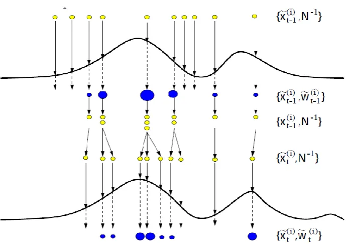
and by Arulampalam et al. (2002), and a schematic representation is given in Figure 1.

At the first step of the algorithm (sampling) 𝑁 random particles (samples) are drawn

from a proposal distribution. These particles are then propagated through the nonlinear

system and are subsequently associated with weights 𝑊̃ according to their fitness, i.e.

equation (4). This step is known as importance sampling. Subsequently, a resampling of

particles with respect to their associated weights is carried out, as a result of which

particles with high weights are split into a number of unweighted particles and particles

with low weights are eliminated. Finally, the introduction of a random noise to the

group of particles at the third step results in local variety in the samples. This process is

visualised in the fourth row of particles in Figure 1. Since, this step provides an

unweighted distribution of particles that mimic the prior distribution, it is referred to as

Figure 1. Illustration of the three stages of importance sampling, resampling, and

prediction in PF, figure from van der Merwe et al. (2000)

In the present study, the application of PF for parameter tracking is of particular

interest. Given a car-following model and a set of data, one can update the estimates of

model parameters upon the receipt of new data. As a result, one will obtain

time-varying estimates of the model parameters. Naturally, these time-time-varying estimates

cannot be used for modelling and simulation purposes, but they can provide a good

insight into some of the very important model characteristics that may otherwise remain

hidden in cumulative error terms. In particular, in simulation-based applications the

parameters are constant, and hence the use of a parameter tracking method gives

information about how a model parameter should deviate from its nominal value to

compensate for modelling flaws. This concept is closely related to model-based fault

detection (Isermann 1984, Venkatasubramaniana, et al. 2003). There is a possibility that

in some cases general patterns in changes of the model parameters are observed (e.g.

driving phase), and this type of information can then be used to improve the quality of

modelling and simulation.

3. Methodology

In this section PF is applied to simulated data to investigate the extent to which the

properties of the adaptive driving can be identified using this method. The section first

introduces the simulated dataset, and then goes on to present the results of the

application. The choice of the objective function for the calibration is also described,

and a simple method for the discretisation of the estimates is proposed. The

discretisation of the dynamic estimates is an important step in the interpretation of the

raw estimates obtained initially and in the linkage of the changes in the model

parameters to the traffic conditions.

3.1 Simulated dataset

In this section the application of particle filtering to simulated data is investigated to

illustrate the extent to which this method can be utilised for the purpose of

“meaningful” parameter tracking in car-following models. The additional constraint

arising from the term “meaningful” refers to the fact that, sometimes by calibrating a

number of model parameters simultaneously, an error in the estimate of one model

parameter may be compensated by an error in another. This could happen due to the

existence of correlation between model parameters and the fact that the information

available is less than what is required for the determination of the unknowns uniquely,

thus causing erroneous tracking of model parameters.

For the data simulation, the trajectories of a specific vehicle from the enhanced

NGSIM I-80 dataset (Montanino and Punzo 2013) were selected. The NGSIM I-80

stretch of an interstate freeway in the San Francisco Bay area, CA (Halkias and Colyar

2006), and the enhanced dataset has been made available by the MULTITUDE project

(Montanino and Punzo 2013). The selected trajectories were then used to generate

trajectories for follower vehicles with the IDM model proposed by Treiber, Hennecke

and Helbing (2000), and a specific parameter profile was used for this purpose. In the

profile used, certain parameters were varied at certain points in time, and particle

filtering was applied to the simulated trajectories to generate dynamic estimates of the

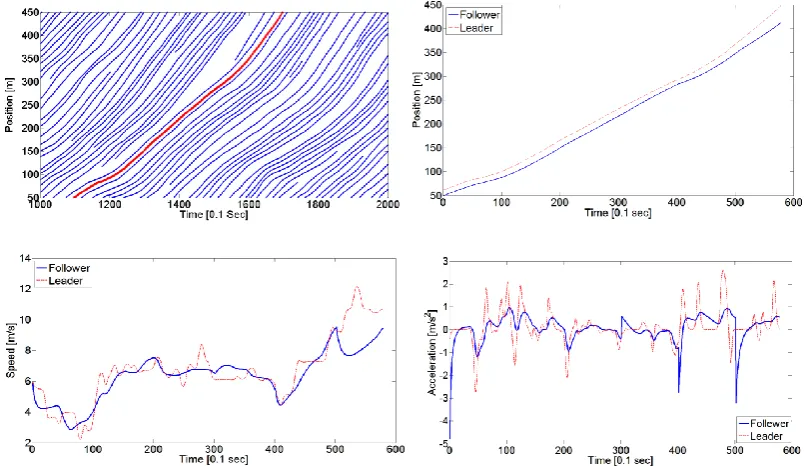
model parameters. Figure 2 illustrates the trajectories used for the leader vehicle.

Figure 2. a) Trajectory of the lead vehicle selected from NGSIM data Lane 2 b,c,d)

Position trajectories, velocities, and accelerations of the lead vehicle and synthetized

follower in dashed red line and blue line respectively

The parameter profiles used for the simulation of the trajectories shown were as

follows: the default model parameters reported by Treiber, Hennecke and Helbing

(2000) were used up to Time = 30 𝑠 , i.e. 𝑎 = 0.73_𝑠𝑚₂, 𝑏 = 1.67_𝑠𝑚₂, 𝑣_𝑑 = 33.3𝑚_𝑠, 𝛿 = 4,

changed to the given values: 𝑏0 = 1.5𝑚_𝑠2, 𝑎0 = 1

𝑚

𝑠2, 𝑣𝑑 = 60

𝑚

𝑠 , 𝑇 = 0.5 𝑠. As such,

the simulation includes the case of having erroneous estimates for some of the model

parameters while another one is being tracked. Additionally, the value of the parameter

𝑇 changes again to the values 𝑇 = 1 𝑠 and 𝑇 = 3 s at time points 𝑡 = 40 𝑠 and 𝑡 =

50 𝑠, respectively.

3.2 Sensitivity analysis

One important consideration in the model calibration is addressing the question of how

the dataset used reflects the characteristics of the model parameters. This is especially

of importance in models, such as IDM, where some degree of orthogonality between

model parameters exists, and different model parameters are best set according to

different types of data in different regimes of driving (Treiber and Kesting 2013). If

this question is not addressed, misleading estimates of model parameters or unnecessary

high computational complexity may result (Ciuffo, Punzo and Mon 2014).

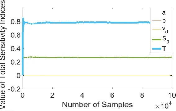
Global sensitivity analysis is used for this purpose, and the more representative

“total sensitivity indices” are used, that capture the impact of parameters across all the

feasible regions in the hyperspace of parameter values (Ciuffo, Punzo and Mon 2014,

Saltelli, et al. 2010, Jacques , Lavergne and Devictor 2006). Figure 3 illustrates the

results for total sensitivity as a function of the number of samples used for the same

trajectory as above. As expected, the results for other vehicles were also found to be

consistent with the ones illustrated, as well as those reported by Ciuffo, Punzo and Mon

(2014). The parameter related to headway, 𝑇, has the highest impact with a total

sensitivity index value of 0.788, and the parameter related to spacing in jam traffic, 𝑠₀,

has the second highest impact, with a total sensitivity index value of 0.268. The rest of

coinciding with the x-axis. The upper boundary (UB) and lower boundary (LB) values

for parameters are given in Table 1.

Figure 3. Total sensitivity indices for the simulation scenario

Table 1 Lower and upper boundary

Parameters LB UB

𝒂 1 3

𝒃 1 3

𝑽𝒅 20 50

𝒔_𝟎 2 10

𝑻 0.5 3

As pointed out by Ciuffo, Punzo and Mon (2014), since the assumption of

parameter independence for such models is unlikely to hold, the results may be subject

to bias. Nonetheless, the conclusions were also verified through a local sensitivity

analysis around the calibrated parameter values, as well as through investigation of the

tracking. Furthermore, an additional justification to the choice of the parameter used in

this study is the physical meaning of it.

3.3 Application of particle filtering to simulated data

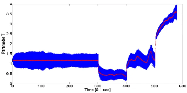
Figure 4 shows the results of the application of particle filtering to the simulated dataset.

For this purpose, all of the model parameters are set to their default values, except for

parameter T, which is to be estimated dynamically.

As was seen, a reason for focusing on T in parameter tracking is that it was

found that no other parameter was capable of tracking the changes in driving behaviour

for multiple trajectories when selected alone. Also, variations in this model parameter

remain low compared to other model parameters. Furthermore, one of the advantages of

IDM is that the parameters have intuitive meanings, and if one parameter is to be

selected among others representing comfortable deceleration, maximum acceleration,

desired velocity, etc., the choice of parameter T, representing headway, is most sensible.

This parameter was also used in Treiber, Hennecke and Helbing (2000) to generate

variations in traffic conditions, and hence driving behaviour, and by doing so the

empirical data related to the formation of traffic jams were successfully simulated.

Figure 4. The result for estimation of the parameter T. The blue shadow denotes the

It can be seen that up to time 𝑡 = 30 s, the estimation of parameter T is almost

error-free and stable. Also, the subsequent changes at the times 𝑡 = 30 𝑠, 𝑡 = 40 𝑠, and

𝑡 = 50 𝑠 can be identified from Figure 4 by “jumps” in the values of the parameter at

these times, compared to the smooth curves in the intervals between the changes. The

estimations of parameter T at times after 𝑡 = 30 𝑠, unlike before, are unstable and

fluctuate around a certain value. This is due to the fact that beyond time 𝑡 = 30 s, other

model parameters were changed to values other than the ones used in the estimation

process. As a result, the effect of this false estimation needs to be compensated by

overestimations and underestimations of parameter T.

Using the parameter estimation given by the application of particle filtering

(Figure 4), an almost perfect estimation of the spacing (𝑅2 = 0.995), velocity (𝑅2 =

0.993) and acceleration (𝑅2 = 0.91) can be derived, despite the errors in the other

Figure 5. The comparison of real trajectories with simulated trajectories when the

dynamic estimation of the parameter T, given by particle filtering, is used.

It should be noted that the IDM car-following model was used to generate

trajectories for the follower vehicles, and the same car-following model was used in the

calibration process. In the application to real data, this is the equivalent of assuming

knowledge of the model underlying the behaviour of human drivers. Although this is

obviously not the case, the findings of Ossen and Hoogendoorn (2008) may justify use

of such simulated data. Therein, it was found that the characteristics of the followers’

behaviour can be recovered by calibrating a car-following model to the data, even when

the real model is different to the model used for calibration.

3.4 Objective function

The objective function defines a measure of error that is intended to be minimised. For

spacing, speed, and acceleration, in addition to an appropriate error test (functional form

of the defined error), such as root mean square error (RMSe) and root mean square

percentage error (RMSPe), as outlined in numerous studies in the literature (Punzo and

Simonelli 2007, Ossen and Hoogendoorn 2008, Treiber and Kesting 2013, Ranjitkar,

Nakatsuji and Asano 2004).

In Punzo and Simonelli (2007) the inter-vehicle spacing was suggested as the

most reliable MOP. In this work, however, it was found that the best result is obtained

when a combination of errors on spacing, velocity, and acceleration was used in the

objective function instead of a single variable. This is due to the use of the information

available on all variables, which avoids outliers and non-smooth modelled data in any

of the three measures individually. In Ossen and Hoogendoorn (2008), in addition to the

different variables for calibration, the use of a combination of speed and spacing in the

objective function was investigated. Therein, despite the fact that the use of a

combinatory objective function including both the spacing and the velocity was found

to be dependent on the specific model used, it was, concluded that when such prior

information about the model is lacking, the use of an objective function including both

speed and spacing could be advantageous. Here, a uniformly weighted sum of squared

errors of all three variables was used, which is an extension to the suggestion made by

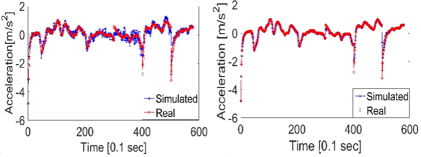
Ossen and Hoogendoorn (2008). The accuracy of the acceleration trajectories in the

NGSIM data is somewhat questionable, as pointed out by Thiemann, Treiber and

Kesting (2008), but excluding the acceleration error between the predicted values and

the real values from the objective function results in randomly fluctuating estimates of

acceleration with unrealistically large values of jerk. This can be avoided by including

the acceleration error in the objective function with a low weight to suppress the

illustrates the simulated acceleration trajectory when the acceleration error is excluded

from the objective function. Although in this case a slight improvement in the simulated

velocity and spacing trajectories is obtained, this improvement comes at the cost of the

acceleration, as can be seen from the figure.

Figure 6. Comparison of the simulated accelerations with the real values when the

acceleration error is: a) excluded from the objective function; b) included in the

objective function.

3.5 Interpreting dynamic parameter estimations

As was shown in Figure 4, although the “jumps” in the values of the model parameters

are visually identifiable, the resulting estimates are much harder to interpret when the

method is applied to real data. This makes the identification of the points where sudden

changes in the model parameters take place difficult, which is due to two reasons: 1) the

actual underlying model is not known in advance; and 2) the changes are much smaller

but more frequent. As one would expect from human drivers, they do not drive in a

crisp and deterministic fashion, and neither do they immediately change their

underlying driving attributes as soon as they reach a different traffic condition; instead a

Hence, a way to identify significant changes and to filter out the smooth

fluctuations from the dynamic model parameter estimate is required. A simple approach

is adopted here for this purpose, whereby the points where maximum changes in the

subsequent values of the parameter under estimation are identified. These points are

referred to as “breaking points”. Following that, the model parameter under

investigation is separately calibrated for each interval between the breaking points.

The detection of breaking points is governed by two conditions, both of which

must hold for a breaking point to exist:

1) The change in the value of model parameter is greater than a certain value,

set to be 0.5 𝑠𝑒𝑐 for parameter 𝑇 here.

2) The distance between each two breaking points is greater than a certain

value. This condition is imposed to avoid frequent changes of the parameter

in a short interval, and its implementation may also be justified by the fact

that frequent and sudden changes in driving behaviour and driving

parameters in a short time interval are highly unlikely among human drivers.

The value of 5 seconds (50 time steps for the NGSIM dataset) is used here.

The application of the proposed discretisation method to the result illustrated in Figure 4

leads to the correct identification of the jumps. Subsequently, parameter T is

recalibrated in separate time intervals: [0, 300], [300, 400], [400, 500], and [500, 600].

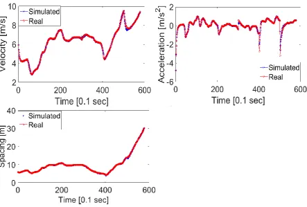
Figure 7. Comparison of the simulated trajectories when averaging between the

breaking points is applied with real results for: a) the estimation of parameter T; b)

spacing; c) speed; d) acceleration.

It can be seen that not only the points where the parameter is changed are

identified correctly, but also that the values of the parameter within corresponding

intervals are estimated with very high accuracy. Hence, the acceleration, velocity, and

spacing trajectories are generated with significantly better accuracy than any

conventional calibration method.

4. Results

In the previous section it was shown that using the particle filtering along with the

proposed discretisation method, the changes in the model parameters can be identified

this method is applied to the NGSIM trajectory dataset to investigate the question of the

identification of the adaptive driving behaviour.

4.1 Application to the NGSIM dataset

The functionality of the proposed method was illustrated using simulated data. In this

section the proposed method is applied to a platoon of nine vehicles driving in the

second lane to investigate the following two issues: 1) whether the assumption of

systematic changes in driving attributes can be validated; and 2) whether these changes

can be identified using car-following models, such as the IDM, and a dynamic system

identification method, such as particle filtering. The procedure is as follows:

1. The five model parameters {𝑎, 𝑏, 𝑣𝑑, 𝑠0, 𝑇} are calibrated using a genetic

algorithm to minimise the sum of squared errors across all the three variables,

namely, spacing, speed, and acceleration (Equation 6).

𝑈 = ∑ ((𝑠_𝑖𝑜𝑏𝑠 _{− 𝑠}

𝑖𝑚𝑜𝑑𝑒𝑙) 2

+ (𝑣_𝑖𝑜𝑏𝑠_{− 𝑣}

𝑖𝑚𝑜𝑑𝑒𝑙) 2

+ (𝑎_𝑖𝑜𝑏𝑠_{− 𝑎}

𝑖

𝑚𝑜𝑑𝑒𝑙₎2₎ 𝑛

𝑖=1 (6)

where: the abbreviations “obs” and “model” denote the observed value and the

modelled value respectively; 𝑛 is the number of sample points; and 𝑠, 𝑣, and 𝑎

denote the spacing, velocity, and acceleration respectively. The objective

function above is the sum of the squared Euclidean distances between the

three-dimensional observed states and the modelled states.

2. At the second step, the parameters {𝑎, 𝑏, 𝑣𝑑, 𝑠0} are fixed to their calibrated

values, while parameter 𝑇 is being tracked given the lead vehicle’s trajectory

and the real trajectory of the follower vehicle. The calibrated values for all the

3. The dynamic estimates of parameter 𝑇 in several runs are then analysed using

the method described in Section 3.5 to identify the breaking points.

4. Once the breaking points are identified, parameter 𝑇 is then calibrated once

more for each time interval between the breaking points.

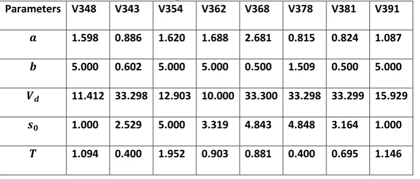
Table 2 The calibrated values of the parameters

Parameters V348 V343 V354 V362 V368 V378 V381 V391

𝒂 1.598 0.886 1.620 1.688 2.681 0.815 0.824 1.087

𝒃 5.000 0.602 5.000 5.000 0.500 1.509 0.500 5.000

𝑽𝒅 11.412 33.298 12.903 10.000 33.300 33.298 33.299 15.929

𝒔_𝟎 1.000 2.529 5.000 3.319 4.843 4.848 3.164 1.000

𝑻 1.094 0.400 1.952 0.903 0.881 0.400 0.695 1.146

All the vehicles observed remain in the platoon for the whole duration of the

experiment, which means that the dynamics are undisturbed by any lane changing

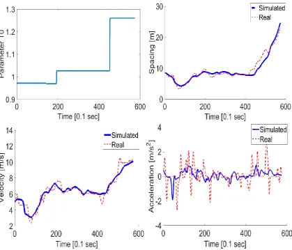
attempts. Figure 8 illustrates the application of the proposed method to one of the

vehicles, and the top-left graph illustrates the discretised parameter estimate.

It should be noted that when applied to the dynamic parameter estimates for real

trajectories, the proposed discretisation method yields breaking points that are less

robust compared to the investigated case of simulated data. In other words, the breaking

points are not always uniquely identified, and while some are detected with a high level

of certainty, others may only be detected in a small percentage of cases. Herein, only

the points that were detected in more than 50% of cases were selected.

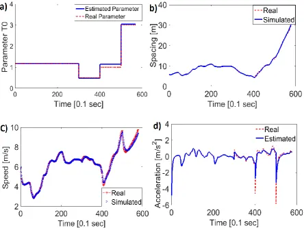
The discretised parameter profile is subsequently used to simulate the driving

speed, and acceleration) with the real states points to the accuracy of the simulated

behaviour. The reason why the acceleration estimates are less solid than the spacing and

speed estimates is due to the low weight of the acceleration variable in the objective

function, as explained earlier.

An interesting finding of this work that can be identified from Figure 8, is the

correlation between the estimate of parameter T, and speed. This will be explained

further in the following section.

Figure 8. Trajectories resulting from application of the proposed method to vehicle no.

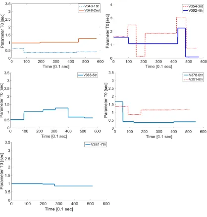
4.2 Analysis of the parameter estimates

Figure 9 illustrates the resulting parameter estimates for the vehicles, based on which

highly accurate estimates of the spacing and velocity trajectories can be obtained. Table

2 summarises the errors in the estimation of velocity and spacing.

Table 3. Measures regarding quality of fit for each of the vehicles in the platoon

V348 V343 V354 V362 V368 V378 V381 V391

Average absolute

error for spacing 0.7366 0.8333 1.8907 1.0251 0.5108 0.7039 0.8268 1.7798

Average absolute

error for speed 0.3885 0.5072 0.6117 0.5066 0.4249 0.5032 0.4805 0.6909

One of the interesting findings is that in the majority of investigated trajectories,

a noticeable relationship between the average speed and estimate of parameter T can be

observed. In particular, from the parameter estimates related to vehicles with IDs 348,

354, 362, and to a lesser extent 343, 378, 391, it can be seen that with the increases in

the average speed, the estimate of parameter 𝑇 increases, and that sudden drops in the

average speed results in drops of parameter 𝑇. The detection of common patterns is an

encouraging result, as it points to a driving phenomenon that the car-following model

fails to account for.

However, interestingly, two other patterns can be observed within the estimates

for this platoon: 1) the inverse relation with the average speed, as in the case of vehicle

no. 368; and 2) irrelevant or no changes in the estimated parameter with respect to

average speed, which is the case for vehicle no. 381. Similar patterns are observed in

many other examined vehicles, and can be most likely be attributed to differences in

driving styles, intentions (such as preparation for performing a lane change), or maybe a

more complicated relation between the average speed and spacing, which could

describe the changes in the model parameter better. Moreover interestingly, in a

statistically significant number of cases, the breaking points are detected at a point in

time where there has been a change in the driving conditions. For instance, considering

breaking points identified correspond to points where: 1) there is a transition from

driving through a shockwave into more homogeneous congested traffic, at about 𝑡 =

20 𝑠; and 2) there is a transition from homogenous congested traffic to a less congested

state where the vehicle starts accelerating at about 𝑡 = 43 𝑠.

It should be acknowledged here that, indeed, the random nature of driving may

be amplified at low speeds and under stop-and-go conditions, and therefore decisive

conclusions can only made when sufficiently large numbers of suitable data are

analysed. A suitable dataset for this purpose would be one consisting of trajectories with

long observation times, where large enough numbers of drivers can be tracked through

different driving conditions. The implementation of the proposed framework on such a

dataset would enable the analysis and interpretation of the jumps in the parameter

values in a broader perspective, and would allow the modification of the method and its

parameters for better performance. The further investigation of these topics and the

application of the method to more trajectories will shed more light on some of these

issues.

5. Conclusions and future work

In this paper, particle filtering was utilised to examine the dynamic behaviour of drivers

in different traffic conditions. In order to interpret the estimates given by the particle

filtering process, a simple discretisation method was used, and promising results from

its application to simulated and real data were obtained. This helped isolate minor

fluctuations, which could be due to the fuzzy and stochastic nature of human driving, or

minor errors in the modelling of car-following behaviour, and to convert the raw

estimates given by the particle filtering process to an interpretable form.

The application of this method to real data delivered interesting results.

speed and the parameter under investigation was observed. This frequent pattern may

point to a common driving behaviour that may not be addressed by the mathematical

structure of the model under investigation. Moreover, two additional patterns were,

interestingly, observed: 1) an inverse relation with the average speed; and 2) no relation

with average speed. Additionally, in a significant number of cases the points that were

detected as breaking points seemed to be the ones where, indeed, a change in the driving

condition took place. Therefore, the employed framework was found to have great

potential in investigating the properties of traffic flow, as well as in examining the

robustness and performance of car-following models.

In future work, the application of suitable clustering methods, such as

consolidated fuzzy clustering (Ma and Andréasson 2007) will be considered for

grouping the estimation results. Moreover, due to the stochastic nature of particle

filtering, the values of the breaking points identified are subject to changes in

consecutive runs. The uncertainty arising from this issue could be tackled by calculating

confidence intervals for these values. Finally, in order to draw reliable conclusions

about how driving behaviour may change with reference to car-following models, an

analysis of larger groups of trajectory data needs to be carried out.

References

Ahmed, K. I. 1999. “Modeling drivers' acceleration and lane changing behavior”PhD

Thesis, Massachusetts Institute of Technology.

Arulampalam, M. S., S. Maskell, N. Gordon , and T. Clapp. 2002. “A tutorial on

particle filters for online nonlinear/non-Gaussian Bayesian tracking.” IEEE

Brackstone, M., and M. McDonald. 1999. “Car-following: a historical review.”

Transportation Research Part F: Traffic Psychology and Behaviour 2, no. 4:

181–196.

Ciuffo, B., V. Punzo, and M. Mon. 2014. “Global sensitivity analysis techniques to

simplify the calibration of traffic simulation models. Methodology and

application to the IDM car-following model.” IET Intelligent Transport Systems

8, no. 5: 479 – 489.

Fritzsche, H.T. 1994. “A model for traffic simulation.” Traffic Engineering and

Control: 317–321.

Halkias, John, and James Colyar. 2006. NGSIM Interstate 80 Freeway Dataset.

Washington, DC, USA: US Federal Highway Administration,

FHWA-HRT-06-137.

Hoogendoorn, S., S. Ossen, M. Schreuder , and B. Gorte. 2006.“Unscented Particle

Filter for Delayed Car-Following Models Estimation.” Proceedings of the IEEE

ITSC 2006 IEEE Intelligent Transportation Systems Conference. Toronto,

Canada.

Isermann, R. 1984. “Process Fault Detection Based on Modeling and Estimation

Methods-A Survey.” Automatica 20, no. 4: 387–404.

Jacques , J., C. Lavergne, and N. Devictor. 2006. “Sensitivity analysis in presence of

model uncertainty and correlated inputs.” Reliability Engineering & System

Safety 91, no. 10-11: 1126–1134.

Kesting, A., and M. Treiber. 2009. “Calibrating Car-Following Models by Using

Trajectory Data: Methodological Study.” Transportation Research Record:

Ma, Xiaoliang , and I. Andréasson. 2007. “Behavior Measurement, Analysis, and

Regime Classification in Car Following.” IEEE TRANSACTIONS ON

INTELLIGENT TRANSPORTATION SYSTEMS 8, no. 1: 144-156.

Montanino, M., and V. Punzo. 2013. “Making NGSIM Data Usable For Studies On

Traffic Flow Theory.” Transportation Research Record: 99-111.

Montanino, M., and V. Punzo. 2013. Reconstructed NGSIM I80-1. COST ACTION

TU0903 - MULTITUDE. http://www.multitude-project.eu/exchange/101.html.

Munoz, J. C., and C. F. Daganzo. 2002. “MOVING BOTTLENECKS: A THEORY

GROUNDED ON EXPERIMENTAL OBSERVATION.” Transportation and

Traffic Theory in the 21st Century. Proceedings of the 15th International

Symposium on Transportation and Traffic Theory. Adelaide, Australia. 441-461.

Ossen , S., and S. Hoogendoorn. 2008. Calibrating car-following models using

microscopic trajectory data. Delft, Netherlands: Delft University of Technology.

Ossen, S., and S. P. Hoogendoorn. 2007. “Car-following behavior analysis from

microscopic trajectory data.” Transportation Research Record: Journal of the

Transportation Research Board Volume 1934 / 2005 Traffic Flow Theory 2005:

13-21.

Punzo, V., and F. Simonelli. 2007. “Analysis and comparison of microscopic traffic

flow models with real traffic microscopic data.” Transportation Research

Record: Journal of the Transportation Research Board 1934, no. 1: 53-63.

Ranjitkar, P., T. Nakatsuji, and M. Asano. 2004. “Performance Evaluation of

Microscopic Traffic Flow Models with Test Track Data.” Transportation

Research Record: Journal of the Transportation Research Board 1876 , no. 1:

Saltelli, A., P. Annoni, I. Azzini, F. Campolongo, M. Ratto, and S. Taranto. 2010.

“Variance based sensitivity analysis of model output. Design and estimator for

the total sensitivity index.” Computer Physics Communications 181, no. 2: 259–

270.

Thiemann, C., M. Treiber , and A. Kesting. 2008. “Estimating Acceleration and

Lane-Changing Dynamics Based on NGSIM Trajectory Data.” Transportation

Research Record: Journal of the Transportation Research Board 2088: 90-101.

Treiber, M., A. Hennecke, and D. Helbing. 2000. “Congested traffic states in empirical

observations and microscopic simulations.” Physical Review E 62, no. 2 : 1805–

1824.

Treiber, M., A. Kesting, and D. Helbing. 2006. “Understanding widely scattered traffic

flows, the capacity drop, and platoons as effects of variance-driven time gaps.”

Phys. Rev. E 74, no. 1: 016123.

Treiber, M., and A. Kesting. 2013. “Microscopic Calibration and Validation of

Car-Following Models – A Systematic Approach.” 20th International Symposium on

Transportation and Traffic Theory (ISTTT 2013). Noordwijk, Netherlands, 922–

939.

van der Merwe, R., A. Doucet , J . F. de Freitas, and E. Wan. 2000. The unscented

particle filter, Technical Report CUED/F-INFENG/TR 380, . Cambridge

University Engineering Department.

Venkatasubramaniana, V., R. Rengas, K. Yinc, and S. N. Kavurid. 2003. “A review of

process fault detection and diagnosis: Part I: Quantitative model-based

Wiedemann, R. 1974. Simulation des Strassenverkehrsflusses. Karlsruhe, Germany:

Schriftenreihe des Instituts für Verkehrswesen der Universität Karlsruhe, Band

8.

Wilson, R. E., and J. A. Ward. 2011. “Car-following models: fifty years of linear

stability analysis – a mathematical perspective.” Transportation Planning and

Technology 34, no. 1: 3-18.

Yang, Q., and H. N. Koutsopoulos. 1996. “A microscopic traffic simulator for

evaluation of dynamic traffic management systems.” Transportation Research C