ABSTRACT
CHEN, MICHAEL. Electromagnetic Energy Localization in Random Mediums. (Under the direction of Michael Steer.)
This dissertation investigates the electromagnetic (EM) scattering of microwave excita-tions in energetic composites, specifically RDX (cyclotrimethylene trinitramine). Of interest is the presence of electric field peaks in these mediums with insight into the potential of a microwave neutralization system for explosives. Such mediums are characterized by large numbers of crystals with sizes on the scale of hundreds of microns, a small fraction of the wavelength of the incident microwave excitation, and an explosive device comprised of many millions of crystals. Furthermore, the critical features in the initiation process are electric field peaks that have a size that is a further fraction of that of the crystals, and dura-tions which are picoseconds long. The number and size of crystals, and the required time and space resolutions make exhaustive re-creation and EM simulation of these mediums extremely time-consuming and infeasible without abstraction. This work develops new, efficient and accurate methods to reduce the time required to perform EM simulation of large volumes of energetic composites.
field behavior, a range of abstractions of crystals is considered to determine the minimum complexity which correctly models field peaking. These abstractions are compared to the more realistic structure of non-uniform crystals placed using a physics based script. It is determined that a medium of randomly rotated and positioned cubes is the best model, offering improved speeds while maintaining the majority of the field localization phenomenon. The presence of hotspots is seen to be heavily influenced by local geometry, with the presence of multiple corners and edges resulting in the highest fields. Peak fields eight times that of the incident excitation are observed.
Finally, a coupling of the electric field behavior into thermal heating is performed via a simulation of dielectric heating and thermal conduction. Locations of high temperature in an RDX-estane composite are tracked over 20 ms for a 1 MV/m sinusoidal excitation, with peak temperature increases of over 75 K. It is observed that while locations of highest electric field do display higher than average temperatures, the higher dielectric loss of the estane binder results in the regions of highest temperature being locations where binder density is high. It is found that regions of high binder density have higher temperatures overall. Still, the highest field locations generally correspond to areas of high temperature. With the compounded effects of electric field and temperature, these locations will have a lower threshold for initiation. than would be suggested by the separate effects.
© Copyright 2017 by Michael Chen
Electromagnetic Energy Localization in Random Mediums
by Michael Chen
A dissertation submitted to the Graduate Faculty of North Carolina State University
in partial fulfillment of the requirements for the Degree of
Doctor of Philosophy
Electrical Engineering
Raleigh, North Carolina
2017
APPROVED BY:
Jacob Adams David Aspnes
Mohammed Zikry Michael Steer
DEDICATION
BIOGRAPHY
ACKNOWLEDGEMENTS
Thanks to Austin, Ian, Matt, Bryan and Nehal for the camaraderie. Thanks to Leland and Tim for making things easy.
Thanks to Spencer Johnson and Professor Adams for the pep talks.
Thanks to Professors Zikry and Aspnes for the discussions in fields I’m less than confident in.
Thanks to Dr. Steer for all of the above, and his endless supply of patience.
TABLE OF CONTENTS
LIST OF TABLES . . . viii
LIST OF FIGURES. . . ix
Chapter 1 Introduction. . . 1
1.1 Overview . . . 1
1.2 Motivation . . . 2
1.2.1 Standoff Excitation of Explosives . . . 3
1.2.2 Creation of a Microwave System . . . 4
1.2.3 Other Applications . . . 5
1.3 Approach . . . 6
1.4 Outline . . . 7
Chapter 2 Literature Review . . . 10
2.1 Introduction . . . 10
2.2 Bulk Characterization of Random Mediums . . . 11
2.2.1 Effects on Communications . . . 11
2.2.2 Sensing and Imaging . . . 12
2.3 Excitation of Energetic Materials . . . 13
2.3.1 Macroscopic Investigations . . . 15
2.3.2 Mesoscopic Investigations . . . 17
2.3.3 Microscopic Investigations . . . 18
2.4 Summary . . . 19
Chapter 3 Effective Permittivity . . . 22
3.1 Introduction . . . 22
3.2 Established Effective Medium Approximations . . . 24
3.2.1 Maxwell-Garnett Effective Medium Approximation . . . 24
3.2.2 Bruggeman’s Model . . . 25
3.2.3 Wiener Bounds . . . 26
3.2.4 Hashin-Shtrikman Bounds . . . 28
3.2.5 Section Summary . . . 29
3.3 Preliminary Estimates . . . 29
3.4 Method . . . 31
3.4.1 Simulation Setup . . . 32
3.4.2 Computing Resources . . . 32
3.4.3 Types of Composite Mediums Used . . . 33
3.4.4 Generation of a Composite Medium . . . 34
3.4.6 Section Summary . . . 38
3.5 Results . . . 38
3.5.1 Slabs . . . 39
3.5.2 Spheres . . . 42
3.5.3 Randomly Rotated Cubes . . . 42
3.5.4 Overview of Other Structures . . . 47
3.5.5 Section Summary . . . 48
3.6 Chapter Summary . . . 48
3.7 Conclusion . . . 50
Chapter 4 Abstraction of Inclusions . . . 52
4.1 Introduction . . . 52
4.2 Method of Simulation . . . 54
4.2.1 Simulation Details . . . 55
4.2.2 Meshing . . . 57
4.2.3 Choice of Abstraction . . . 59
4.2.4 Section Summary . . . 63
4.3 Scaling of Peak Field Magnitude . . . 66
4.4 Initial Results . . . 67
4.4.1 Accuracy of Abstractions . . . 67
4.4.2 Resource Efficiency of Abstractions . . . 72
4.4.3 Section Summary . . . 73
4.5 Extension of Case 5 . . . 76
4.5.1 Decomposition of Case 5 . . . 76
4.5.2 Intersection of Inclusions . . . 84
4.5.3 Section Summary . . . 89
4.6 Limitations . . . 90
4.6.1 Excitation . . . 90
4.6.2 Sample Sizes . . . 91
4.6.3 Accuracy of Method . . . 92
4.7 Validation . . . 93
4.8 Chapter Summary . . . 93
4.9 Conclusion . . . 95
Chapter 5 Microwave-Induced Thermal Behavior . . . 99
5.1 Introduction . . . 99
5.2 Approach . . . 101
5.3.4 Methods-EM Thermal Coupling . . . 107
5.3.5 Section Summary . . . 109
5.4 Results . . . 110
5.4.1 EM Results . . . 110
5.4.2 Dielectric Heating per Cycle . . . 112
5.4.3 Conduction Heat Transfer over Time . . . 114
5.4.4 Behavior within Inclusions . . . 120
5.4.5 Section Summary . . . 120
5.5 Graphical Analysis of Thermal Progression . . . 123
5.5.1 Distribution . . . 129
5.6 Chapter Summary/Discussion . . . 131
5.7 Comparison to Previous Studies . . . 133
5.8 Conclusion . . . 134
Chapter 6 Conclusion . . . 137
6.1 Summary of Chapters . . . 137
6.1.1 Effective Permittivity . . . 138
6.1.2 Abstraction of Inclusions . . . 139
6.1.3 Microwave-Induced Thermal Behavior . . . 142
6.2 Overall Conclusions . . . 144
6.2.1 Potential of a Microwave System . . . 145
6.3 Future Work . . . 147
6.3.1 Extensions of this Work . . . 147
6.3.2 System Level Considerations . . . 148
BIBLIOGRAPHY . . . 149
APPENDICES . . . 157
Appendix A FDTD Structure Generation . . . 158
A.1 Cubical Inclusions . . . 159
A.2 Spherical Inclusions . . . 167
Appendix B MATLAB Effective Permittivity Calculator . . . 172
Appendix C Bucket Script . . . 174
Appendix D MATLAB Thermal Scripts . . . 202
D.1 Dielectric Heating . . . 203
LIST OF TABLES
Table 3.1 Extracted effective permittivity values for expanded set of structures, simulated with a filling factor of 30%. . . 47
Table 4.1 Summary of Case Properties . . . 63 Table 4.2 Simulation runtimes and memory requirements for each level of
ab-straction or Case. The memory is the combined CPU (up to 64 GiB) and GPU (up to 10 GiB) memory used in the EM simulation. The mem-ory required for mesh generation determines the maximum memmem-ory required. . . 74 Table 4.3 Inclusion properties for the variations of Case 5 described and
simu-lated in Section 4.5 . . . 90
LIST OF FIGURES
Figure 2.1 Silver/Gold hollow nanostar. In medical applications, these are added to target areas to enhance response to imaging tools. From[31]. . . . 14 Figure 2.2 Examples of structures used in previous investigations of initation
mechanismsat the macro, meso and micro-scale. . . 16
Figure 3.1 Wiener Bounds, maximum and minimum conductivity examples, the direction of the arrow represents the direction of the propagation of the excitation wave,+x. . . 27 Figure 3.2 Preliminary estimates of effective permittivity from various models
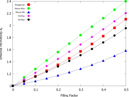
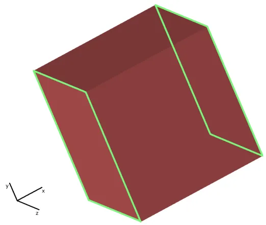
and approximations over range of filling factors from 0 to 50%. The Bruggeman model is calculated from Eqn. 3.2, the Wiener Bounds calculated from Equation 3.4, and the HS Bounds from Equation 3.5. 30 Figure 3.3 Waveguide simulation setup, scattering medium is in red, waveguide
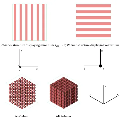
ports are outlined in green. . . 33 Figure 3.4 Simulation structure examples. . . 35 Figure 3.5 Inclusion dimensions for the medium of cubic inclusions and medium
of spherical inclusions described in Figure Figure 3.4 across range of fill factors from 0–34% . . . 36 Figure 3.6 Slab thickness for the composite mediums of Figure 3.7. In all cases,
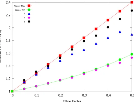
six slabs in total are evenly spaced in the medium . . . 37 Figure 3.7 Extracted permittivities from simulation of slab structures withx,y
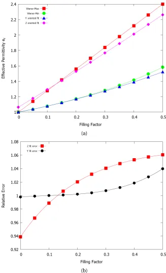
andzorientation, as described in Section 3.5.1. Filling factor varied at 10 evenly spaced points between 0 and 50%. Maximum and minimum Wiener bounds from Eqn. 3.4 included for comparison. . . 40 Figure 3.8 Extracted permittivities: (a) Best fit lines for the extracted
permit-tivities of the y– andz–oriented slabs plotted in Fig. 3.7. Wiener Bounds included for comparison (b) Relative error between the best fit lines and the Wiener Bounds.z–oriented slabs are compared to the maximum bound, whiley–oriented slabs are compared to the minimum. . . 41 Figure 3.9 Extracted relative effective permittivity for a medium with inclusions
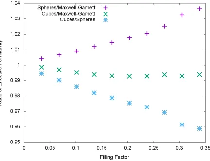
Figure 3.10 Extracted relative effective permittivity for a medium with inclusions comprised of randomly rotated cubes created with the method de-scribed in Section 3.4.4, with filling factors at 10 evenly spaced points between 0 and 34%. Individual plot points are average values from 5 separate random runs. The HS bounds are plotted between 0 and 50% for comparison. . . 45 Figure 3.11 Comparison of extracted permittivities of medium comprised of
cu-bic inclusions from Fig. 3.10, medium comprised of spherical inclu-sions from Fig. 3.9, and Maxwell-Garnett approximation from Eqn. 3.1. . . 46 Figure 4.1 Simulation structure with excitation propagating from−xto+x. The
incident EM field has an E-field polarization in the z direction. Scatter-ing medium fillScatter-ing factor is reduced for clarity and not representative of actual packing density of simulation medium. . . 56 Figure 4.2 Excitation pulse: (a) with a center frequency of 15 GHz and width of
180 ps; and (b) frequency content. . . 58 Figure 4.3 Meshing comparison showing the difficulty the FDTD method
en-counters meshing spherical shapes, observable by the staircase effect on the sphere’s surface. Mesh only images included for improved visibility. . . 60 Figure 4.4 SEM image of RDX Crystals, showing edges and corners of
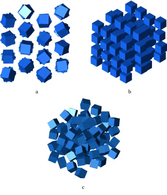
inclu-sions. Crystals can be seen ranging from approximately 10 to over 50 microns in size. From[70]. . . 61 Figure 4.5 Various simulation structures Case 1 is a single sphere; Case 2 is a
single randomly oriented cube; Case 3 is an array of cubes on a grid; Case 4 is an array of randomly arranged spheres; and Case 5 is an array of randomly arranged cubes. . . 64 Figure 4.6 Case 6, generated by the Bucket script of falling and shaken randomly
generated crystals as described in Section 4.2.3, filling factor as simu-lated. . . 65 Figure 4.7 Peak field values for the waveform in Figure 4.2, and the abstractions
in Figures??and 4.6 for varying mesh density and a characteristic dimension of 100u pµm. . . 69 Figure 4.8 Peak field values for the waveform in Figure 4.2, and the abstractions
Figure 4.10 Peak field values for the waveform in Figure 4.2 for Cases 5R, 5T and 5RT in Figure 4.9 for varying mesh density and a characteristic dimension of 100µm. . . 78 Figure 4.11 95% scattering bounds of the scatter plot of 4.10 for varying mesh
den-sity and a characteristic dimension of 100µm, center point defined by best fit line. . . 80 Figure 4.12 Fit lines of the range of the scattering bounds of Figure 4.11 for Case
5R, 5T and 5RT. Individual points represent the magnitude of the single sided 95% scattering bound at the points mesh densities in Figure 4.11. One very high peak field scattering range is recorded at the lowest meshing density for the Case 5RT simulations. This is an anomaly due to low mesh resolution. . . 82 Figure 4.13 Relative increases in peak field of Cases 5R, 5T and 5RT from Figure
4.9, defined as the increase in peak field values at each mesh density relative to the peak field strength for Case of the regular cubes, Case 3. The product of the increases of Case 5R and Case 5T is also included. 83 Figure 4.14 Illustration of randomly generated cubes (a) allowed to intersect and
(b) reoriented to avoid intersection . . . 84 Figure 4.15 Comparison of peak field values of Case 5I, the modified version of
Case 5 with intersection allowed with those of Case 6, from Figure 4.6 over varying mesh density. The results are the average of 25 random realizations of Case 5I and 10 random realizations of Case 6. The peak incident E-field is 1 V/m, as shown in Figure 4.2 . . . 86 Figure 4.16 Field cross section comparing peak field geometries of Case 5 and
Case 5I. The colorbar for both figures represents the electric field strength in V/m . . . 87 Figure 4.17 Field cross section comparing peak field geometries of Case 3, Case
5R, and Case 5T . . . 88 Figure 5.1 Simulation structure (shown here in xFDTD). . . 105 Figure 5.2 Windowed sinewave showing the first two cycles of the excitation. . . 109 Figure 5.3 Cross section of peak electric field strength in MV/m, maximum value
overx projected ontoy-z plane. . . 111 Figure 5.4 Cross section of heat transfer density over two periods of excitation
sinusoid in J/m3, maximum value overx projected ontoy-z plane. . 113 Figure 5.5 Thermal status at 1 million cycles (60.6µs) projected in they-zplane:
Figure 5.6 Thermal status at 10 million cycles (606µs) projected in the y-z
plane: (a) temperature in kelvin; and (b) temperature change due to conduction in K/µs. The circles in (a) identify five locations of interest over the course of the simulation. . . 117 Figure 5.7 Thermal status at 30 million RF cycles (1.82 ms) projected in they-z
plane: (a) temperature in kelvin; and (b) temperature change due to conduction in K/µs. The circles in (a) identify five locations of interest over the course of the simulation. . . 118 Figure 5.8 Thermal status at 60 million RF cycles (3.64 ms) projected in they-z
plane: (a) temperature in kelvin; and (b) temperature change due to conduction in K/µs. The circles in (a) identify five locations of interest over the course of the simulation. . . 119 Figure 5.9 Single dx cross section, chosen at 30000 cycles, showing cold interior
of inclusions, temperature in Kelvin . . . 121 Figure 5.10 Single dx cross section, chosen at 30000 cycles, showing conduction
heat transfer within inclusions. Heat transfer in mJ/m3 . . . 122 Figure 5.11 Absolute temperature (a) across entire medium (b) of five locations
of interest, average temperature across structure for comparison, recorded over entire simulation . . . 124 Figure 5.12 Local geometries of locations of interest . . . 126 Figure 5.13 Total heating rate at each location of interest over entire simulation,
bulk for comparison . . . 127 Figure 5.14 Conduction heating rate at each location of interest, the bulk
re-sponse is shown for comparison . . . 128 Figure 5.15 Total heating rate of RDX and binder due to conduction over entire
simulation . . . 129 Figure 5.16 Histograms of temperature distribution in: (a) RDX and; (b) binder
Chapter
1
Introduction
1.1
Overview
Energetic materials, which give explosive devices their destructive capabilities, release energy through the breaking of many chemical bonds in a chain reaction. In this way, they are inherently unstable. This instability can be undesirable, as in the case of an unexpected shock which causes accidental, unwanted initiation. They may also be advantageous, as in the remote, non-contacting initiation of explosive devices via a distant source. In particular, it is possible to control the chain-reaction, causing energy to release at a slower rate, which results in the deflagration of the material, instead of a more violent detonation[1]. This manifests as a slow burning of the material, effectively neutralizing the device. Deflagration is less common in acoustically or mechanically excited explosives, and believed to be due to the ability of EM and thermal excitations to introduce energy at a slower rate.
acoustic, mechanical and thermal excitation have shown consistent, reproducible success in initiating energetic materials. However, deflagration via purely electromagnetic (EM) excitation is relatively inconsistent and/or inefficient, and poorly understood. In particular, EM excitation sources in the microwave regime have been shown to cause initiation, but detailed results have proven difficult to record[2].
A key factor in the neutralization of these materials is the creation of hotspots, areas of particularly high stress. This stress can be the result of mechanical and acoustic interactions or chemical processes. However, in the case of EM excitation, the two main quantities relevant to hotspot formation are the electric field itself (as the materials in question are typically non-magnetic), and the heat and temperature changes generated through losses in electric field energy. High electric field strengths and changes in temperature have both been shown to cause or facilitate the initiation of energetic material[3],[4]. Therefore, it is imperative that the generation of these hotspots is better understood.
The end goal of this line of research is the development of a microwave system which is capable of reliably causing initiation of energetic materials, without knowledge of the material’s exact geometry.
1.2
Motivation
1.2.1
Standoff Excitation of Explosives
The primary motivation of this work is the standoff excitation of explosives, particularly homemade, sub-military grade explosives. The structures studied in this work will bear greater resemblance to these lower quality explosives than military grade explosives, which feature significantly less randomness in their geometry, while improvised explosives are commonly of this lower quality.
This work will also focus exclusively on microwave frequency sources in the range of 3 to 30 GHz. While high-frequency laser sources have shown a higher degree of reliability in reproducing initiation, microwave sources offer several distinct advantages. The microwave excitations in question are approximately 1000 times lower in frequency than the onset of the infrared portion of the frequency spectrum, allowing for larger areas of illumination. With beamwidth inversely related to the frequency of the source, Gaussian laser sources offer beamwidths in the micron range, while very high power microwave sources have been shown to possess much larger beam areas.
In addition, a wide variety of nonmetal substances are relatively transparent at mi-crowave frequencies, while frequencies at infrared and above struggle to penetrate many common materials used in the covering or containment of explosives. This also allows microwaves to pass through these materials non-destructively, where high powered laser sources may cause heat damage and be unable to pass through coverings.
the relatively ineffective conversion of energy, as nearly all studies suggest a correlation between source strength and the effectiveness of the excitation.
1.2.2
Creation of a Microwave System
To overcome these difficulties and fully exploit the possibility of the neutralization of en-ergetic materials with a microwave excitation, it is necessary to gain a detailed insight into the behavior of microwaves in these mediums and their effects. Several specific chal-lenges in understanding must be overcome to facilitate the development of a microwave neutralization system for these materials.
One challenge is the size of the inclusions1in these materials relative to the wavelength
of microwaves. Linear dimensions are typically on the scale of tens to hundreds of microns
[5]–[8], which is far larger than wavelengths at laser frequencies, but at least an order of
magnitude less than microwave wavelengths. In situations such as this, scattering effects of individual inclusions are sometimes considered negligible, and the medium as a whole defined as an effective permittivity.
The concept of effective permittivity is one possibility for characterization of a medium. However, as it has been shown that ignition locations of energetic materials is on the micron scale[5], and may be caused by behavior at even smaller scales[9], it may also be necessary to understand the behavior at the sub-inclusion level. Effective permittivity characterizations would be unable to describe behavior at these levels, as the onset of initiation is not a bulk effect. Rather, localized extremes in field and temperature over
minute intervals of time and space are the triggering mechanism.
Successful development of the aforementioned microwave initiation system would augment countermeasure capabilities for IEDs. The capabilities of such a system include remote landmine disarmament and neutralization of suicide bombers. Many current meth-ods typically require user input in close proximity of the explosive, an inherently dangerous proposition. Furthermore, a directed microwave excitation system would have little effect on non-explosive materials caught in its beam, limiting collateral damage. High strength fields may damage electronic systems, though this may have its own benefits for a neutral-ization system.
Application of directed energy weapons will almost certainly result in deflagration of an explosive and not in detonation, a preferable outcome. In addition, better understanding of the behavior of microwaves in these materials would assist in the study of complementary initiation mechanisms. This would benefit the development of systems which also utilize acoustic, shock, or thermal excitation systems.
1.2.3
Other Applications
research across many disciplines, application areas for these concepts is expected to greatly increase. Possible subjects include carbon fiber reinforced composites, which utilize ran-dom fibers, characterization of solid rocket fuel, buried structure demolition, as well EM characterization of nanomaterials (nanotubes, walls, stars, etc.).
1.3
Approach
In addition to being strictly regulated, experimental characterization of energetic materials is often impractical, with detailed in situ measurements usually impossible. In addition, successful initiation of the material can have destructive results. This work will focus on various simulation-based approaches capable of obtaining more detailed data. Simulation-driven methods grant the user the flexibility to define data resolutions in both space and time (within computing resource limitations). The disadvantage lies in the long runtimes required to run simulations in the detail required for the purposes of this work.
Three major investigations will be performed:
1. Characterization of effective permittivity
2. Abstraction of medium to generate EM hotspots
3. Analysis of EM-thermal coupling
EM simulations will be performed using Remcom’s xFDTD software, which uses the finite-difference time domain (FDTD) method[10]. FDTD has the advantage of scaling well with increased parallel computing resources relative to other methods. Thermal analysis is done via an in-house MATLAB script – developed specifically for this project – which combines the effects of dielectric heating with conductive diffusion. Structures for simu-lation are defined with the aid of the Bullet Physics software library[11], which is utilized in in-house C++scripts to define the scattering structures. These structures are imported into the other programs for simulation.
1.4
Outline
The goal of this work is to determine the proper level of abstraction to capture energy localization in sub-millimeter scale granular composites, and apply those abstractions to test their validity.
Chapter 2 provides a literature review of topics indirectly related but relevant to the EM initiation of energetic materials, particularly the characterization of and various methods of simulation for EM waves in random mediums, as well as a summary of research in energetic material initiation across multiple disciplines. A brief overview of directly related topics is covered at the beginning of subsequent chapters.
than one-twentieth of a wavelength of the EM excitation may be characterized with an effective permittivity. It is less clear whether this will allow for predictions concerning field peaking. In addition, there are many effective permittivity models. It is not clear which, if any, are adequate for the situation here. The purpose of this chapter is to first determine which effective permittivity model best applies to the composite granular structure and then to determine the peak fields that could be predicted using an effective permittivity model. The field peak fields predicted through this model may be compared to the peak fields determined from more detailed EM simulations in latter chapters. The benefits and drawbacks of the effective permittivity characterization are explored.
Several inadequacies are discovered with the effective permittivity method during the investigations performed in Chapter 3. Chapter 4 investigates the applicability of various lower level abstractions of the medium of energetic material (lower level in this case refers to a lower degree of abstraction, i.e. closer to the actual structure). The goal of this investigation is to determine the abstracted structure which provides significant advantages in setup and simulation runtimes, while maintaining the energy localization of interest. In doing so, the most effective abstraction is obtained, as is insight into the generation of hotspots.
and possible features of interest noted.
The final Chapter ties the observations from the preceding chapters together, providing a summary and suggesting areas for improvement or further investigation.
Chapter
2
Literature Review
2.1
Introduction
2.2
Bulk Characterization of Random Mediums
While sub-wavelength detail into the scattering of electromagnetic waves is an admirable goal for any electromagnetic simulation, it is for many applications sufficient to determine a single, or greatly reduced set of parameters which captures the behavior of interest. This is especially true in communications and sensing, where the overall power of the transmitted or reflected signal is of far greater importance than minute details of the signal’s journey.
2.2.1
Effects on Communications
A significant portion of the studies of electromagnetic propagation in and through random mediums considers the degradation of radar and communications signals in a scattering medium such as the atmosphere or various forms of precipitation. Several factors make this situation relatively simple to analyze. In communications systems the desired metric is the received power at a point beyond the medium – the behavior of the wave within the medium itself is of little interest. Therefore, it is convenient to generate a bulk characterization of the medium focused solely on this metric. In addition, the majority of the mediums that hamper, but still allow the possibility for, radio communications are sparsely populated, reducing the overall complexity of the problem. Finally, the interfering medium is usually a small portion of the total channel, diminishing the impact of near-field effects.
vast number of studies have been performed in this area, across a wide range of frequencies and types of precipitation. Several reviews provide a fairly comprehensive summary of the state of the field over the past half-century[14]–[16]. Most of the work has focused on statistical models which provide acceptable accuracy over a range of conditions. There has also been work performed for specific inclusion shapes, which may then be superimposed to generate results for a custom geometry[17],[18].
A second set of communications challenges in random mediums focuses on electro-magnetic propagation through vegetation canopies. These have also seen analysis as a summation of discretized scatterers[19]. However, as the dominant constituent material in these mediums is water, they may be analyzed in a manner similar to the precipitation[20].
2.2.2
Sensing and Imaging
The study of EM propagation in random mediums also finds application in the field of remote sensing and imaging systems, which often encounter mediums with structures similar to the granular composites in this work. These include various types of soil and sand, as well as packed snow and ice. In these cases, the result of interest is the reflected or backscattered power, in order to determine the composition of the medium under investigation. It is often convenient to characterize the random medium with an effective permittivity. This may be done by Monte-Carlo simulation of many generated random mediums[21],[22], or experimental characterization[23].
Sensing with random mediums also finds application in the analysis of scatter from sea
There have been some studies on the localization of EM energy in composite mediums with scales of size similar to this work[12],[26],[27]. These will be reviewed in Chapter 4. However, a larger number of investigations fall under the category of particle physics and quantum optics. Significant research has been performed in this area on the synthesis of inclusions capable of producing high levels of Surface Enhanced Raman Scattering (SERS). As the Raman scattering effect is generally weak, high field levels are required to create a detectable result. Certain geometries have long been known to produce enhanced field levels for this purpose[28], while noble metals have been shown to generate the highest level of SERS[29].This finds application in biomedical imaging, where the effect can be incorporated into a process which greatly enhances the visibility of certain pathogens[30]. A variety of shapes have been synthesized from silver, gold and platinum which display greatly enhanced fields[31]–[35]. The most prominent among these is the hollow nanostar (HNS)[31],[35], illustrated in Figure 2.1. The combination of the geometry and material of these inclusions can result in a response many orders of magnitude greater than would be observed without their presence[30].
2.3
Excitation of Energetic Materials
Extensive work has been performed on the effects of various excitations on the initiation of energetic materials, especially impact and heat. Multiple cases of successful initiation via these sources have been documented[36],[37]. While electromagnetic have received significantly less attention, several cases of successful initiation by both microwave[2],[38] and laser sources have been recorded[3],[4].
Figure 2.1Silver/Gold hollow nanostar. In medical applications, these are added to target areas
into the macroscopic (bulk), mesoscopic (inclusion), and microscopic (molecular) levels, with different effects dominating at each. Examples of the three levels of scale are presented in Figure 2.2, with the three panels showing a heating experiment for a packed sample of energetic material, an EM-thermal simulation of a collection of circular inclusions, and a molecular dynamics simulation of a single molecule of explosive material.
2.3.1
Macroscopic Investigations
At the macroscopic scale, energetic materials are often excited through heating, with the purpose of initiating explosion or deflagration. This heating can occur via conduction[39],
[40], friction[41]or via an electromagnetic excitation[2],[38],[42]. Such investigations
typically monitor temperatures at several points in the material. Initiation through thermal heating is typically consistent but the time to initiation is highly dependent on the heating rate, with studies having been performed for both slowly heated [40]and flash heated samples[42].
At this scale, experimental measurements are a possibility, although they are typically limited to examining the surface through thermal imaging[41],[43], or through various methods of observing the actual explosion[3],[38],[44]. Approaches using simulation may provide more details within the medium[42]. However, at this scale, simulations are inherently limited to bulk heating.
Microwave excitations have been studied at this scale, due to their ability to pass through most materials relatively unhindered, but these methods have proven to be slow[2]or unreliable[38].
Macroscale – Bulk heating apparatus[39] Mesoscale – Temperature map of circuar inclusions[5]
rate, as well as their interactions with individual molecules at the microscopic level. The main mechanism behind is the heating of the binder[1], as the actual energetic material itself is much more difficult to heat. Unfortunately, the low effective range and beamwidth and these lasers restricts their applicability for standoff excitation. Typical experiments are limited to ranges of a few centimeters or less[45], or requiring the use of systems of mirrors and lenses too focus the beam at the surface of the material[3],[4],[46], limiting their potential for use in real world applications.
2.3.2
Mesoscopic Investigations
Relative to the other scales, it is difficult to obtain a full picture of the situation from a mesoscopic investigation. A macroscopic perspective offers easy access to experimental results, and while these experiments may run over many periods at the excitation frequency, the duration in real time is short. At the opposite end of the spectrum, the very small scale of the microscopic study allows for an in-depth analysis of molecular dynamics or even quantum effects, with a wide range of commercial tools available. However, the mesoscopic situation may help develop understanding the interactions between inclusions, which is not possible at the other two scales.
Pickles et al. examined the structure from an effective permittivity perspective[12],[26]. However, they observed high levels of deep sub-wavelength field localizations in composite mediums. Localizations at a scale of one-hundredth the free space wavelength have been determined in simulation. Perry et al. also examined the EM induced thermal behavior in energetic composites, observing ignition points on the sub-inclusion scale[5].
2.3.3
Microscopic Investigations
Studies at the microscopic level are typically performed from a quantum chemistry per-spective. Similar to the mesoscopic studies, microscopic investigations are entirely done in simulation. The main features of interest here are the covalent bonds between the molecules’ constituent atoms, which break to begin the initiation of the energetic material. Temperature and impact shock are essentially constant over these scales – variation exists in the electric potentials and chemical properties. A typical excitation mechanism is the dropping of the molecule from a height[48].
It may also be the case that multiple types of excitation are coupled, their compounded effects likelihood of initiation to a greater degree than the sum of the individuals. Multiple investigations have explored the relation between impact initiation and the temperature of the energetic material[49],[50]. The general consensus is that the stress from either the impact or thermal energy can increase the energetic materials sensitivity to another stressor. In short, the different excitations work together to induce activity in the material.
[51]. Such investigations are performed from a chemistry perspective, focusing on inherent
potential differences due to charge imbalances. However, it may be possible to induce similar charge balances through an external source.
Work by Wood et al. has investigated the increase in energy of energetic materials due to electromagnetic excitation. They found that frequencies corresponding to the resonant modes were the most efficient at initiating decomposition of the material, though the electromagnetic excitation has a positive effect on decomposition regardless of frequency
[52].
An overarching theme among these microscopic level studies is the importance of hotspots in the initiation process. These various stresses (impact, heat, electric potentials, bond weakness) are not universally present or equal throughout the medium. For these effects to compound, their areas of influence need to overlap. The hotspot sizes of these stresses, can vary greatly, from the sub-molecular scale of the chemical bond to the much larger impact shock area caused by a drop.
2.4
Summary
A significant amount of investigation has been performed concerning electromagnetic waves in random mediums, as well as the excitation of energetic materials with external stimuli. Still, extensive opportunities for further investigation remain.
The studies in electric field localization have focused on nanoscale particles and corre-sponding frequencies, searching for ways to maximize SERS. They are typically performed a semi-classical or quantum perspective, while the methods in this work operate from an entirely classical perspective. In addition, while these SERS studies seek to synthesize a structure to maximize fields, this work seeks to better abstract existing structures which display peak fields.
Regarding the excitation of energetic materials, there exist many studies at the macro-scopic and micromacro-scopic scales. There is, however, a lack of studies at the mesomacro-scopic levels, while those that exist employ significant simplifications or assumptions. While the smaller and larger scales have their merits, it is at this intermediate level where external microwave fields should localize, and therefore at this level which this work must operate.
Chapter
3
Effective Permittivity
3.1
Introduction
In Chapter 1, the problem of the excitation of a granular composite medium by an EM wave was introduced. The major complication in the analysis of this situation is the large number of inclusions, each with its own contribution to the scattering of the incident wave, making an exhaustive analysis extremely time-consuming. To conserve time, studies may be limited to few realizations of the random medium, limiting confidence in the results. The development of a simplified model of the structure which retains the relevant scattering behavior would greatly increase rate at which simulations may be performed, resulting in faster development of insight into the phenomenon.
lations required. While presenting clear drawbacks – this solitary value cannot possibly encapsulate all the information of value – effective permittivity methods have nonetheless remained popular since the first studies of EM propagation through random mediums.
To facilitate the characterization of scattering mediums with an effective permittivity, a variety of experimental, theoretical, and simulational investigations have been performed regarding the matter. Since the final result is to be condensed to a single value, abstracting the medium is a logical intermediary step. Many abstractions have been attempted, ranging from the relatively high–level models involving slabs[53]and cylinders, to relatively lower level attempts with spheres[54]and dipoles[55].
Another possible tradeoff that can be made regards the number of dimensions con-sidered in the problem. The aforementioned slab and cylinder abstractions reduce the dimensionality of the problem to some degree, but still involve analysis in three dimensions. However, extensive analysis has been performed at the 2-dimensional level, with studies leveraging the simplicity offered by rough surfaces[56]and circles[57]. Even 1-dimensional analyses of certain surfaces have proven informative[58].
3.2
Established Effective Medium Approximations
Among the many studies which utilize effective mediums, several effective medium theories or mixing models are commonly utilized. While not as well-suited for specific mediums as customized models, these general models often serve as an initial estimate, or a standard of comparison for a customized model. Whereas customized models often rely on numerical fitting of empirical data, these standard models are derived theoretically. The models in this section will prove valuable for comparison and validation of results.
3.2.1
Maxwell-Garnett Effective Medium Approximation
The Maxwell-Garnett approximation estimates the effective permittivity of a two-phase composite medium as[59]:
"eff="2+3qv"2
"1−"2
"1+2"2−qν("1−"2)
(3.1)
to a fill factor of approximately 35%, around the percolation threshold1for a medium of
spheres[61]. This upper bound of this range sits at approximately the fill factor of interest.
3.2.2
Bruggeman’s Model
A second effective medium model is that of Bruggeman. In its two-phase form it is[62]
q1
"1−"eff "1+2"eff
+q2
"2−"eff "2+2"eff
=0 (3.2)
In Equation (3.2),"1and"2are the permittivities of the medium’s constituent materials, and
q1andq2their respective fill factors. Unlike the Maxwell-Garnett approximation,
Brugge-man’s model does not require the identification of a specific material as the inclusion, and the other as the matrix. The matrix and inclusions are homogenized and treated as a whole in the derivation, making the Bruggeman model perhaps a better embodiment of the effective medium concept.
The Bruggeman model has the advantage of being extendable to mediums with more than two phases by appending additional terms, as well as being more accommodating of shapes. It has also been reported to remain accurate to slightly higher fill factors, up to 50%, comfortably above that of our structure of interest[62]. However, the homogenization technique used is still limited to ellipsoidal shapes.
3.2.3
Wiener Bounds
The Wiener bounds set the upper and lower limit on the conductivity (σ) of a random composite medium. Perhaps not technically an effective medium theory, the bounds still provide a starting point and range for possible values of effective permittivity. Both bound-ing structures are composed of slabs of material rather than inclusions. The upper limit on conductivity is the case of slabs aligned parallel to the propagation direction of the wave, illustrated in Figure 3.1. At the opposing end of the spectrum, the case of slabs aligned perpendicular to the direction of propagation presents the lowest possible conductivity.
One analogy for this behavior is a comparison to a set of connected resistors. The slabs in the maximum conductivity configuration are analogous to a set of resistors in parallel, where all the excitation has a direct path via the material of greatest conductance (lowest value resistor). The overall conductivity is dominated by the most conductive element. Similarly the minimum conductivity configuration is analogous to a set of resistors in series. The excitation must always pass through the least conductive element (highest value resistor). The overall resistance is therefore dominated by the most resistive element.
The conductivity expressions for these bounds take a form similar to those of the resistive networks, and for a two-phase composite is given by[53]
σmin=
1 P2
n=1 qn
σn
≤ σeff ≤
σmax= 2 X
n=1
qnσn
(3.3)
Maximum conductivity structure
Minimum conductivity structure
Figure 3.1Wiener Bounds, maximum and minimum conductivity examples, the direction of the
"max=qν"1+ (1−qν)"2
≥ "eff ≥
"min=
"1"2
qν"2+ (1−qν)"1
(3.4)
Though these bounds are admittedly coarse, they provide a first step sanity check for any results produced.
3.2.4
Hashin-Shtrikman Bounds
A more comprehensive and relevant set of bounds can be found in the work of Hashin and Shtrikman[63]. These bounds are derived from a structure of tightly packed spherical inclusions of varying size, and always fall between the Wiener Bounds, that is, the mini-mum Hashin-Shtrikman (HS) bound is higher than the minimini-mum Wiener Bound while the maximum HS bound is lower than the maximum Wiener Bound. The theory behind the HS bounds is not unique to the study of effective permittivity and is applicable to the characterization of any form of wave propagation through a composite medium. The derivation is significantly more involved than the models of previous sections – their final form with regard to effective permittivity is given by[63]
"min="1+
qν
1
"1−"2 + 1−qν
3"1
≤ "eff ≤
"max="2+
1−qν
1
"2−"1 + qν 3"2
(3.5)
vacuum for the first portion of this work.
In practice, these bounds are in fact the Maxwell-Garnett approximation and its com-plement (with the materials properties of the inclusion and matrix switched). However, the difference in their origin warrants the HS bounds their own mention. This also constrains the effectiveness of the HS bounds to the same range of filling factors as the Maxwell-Garnett approximation.
3.2.5
Section Summary
Several theories which predict the effective permittivity of a composite medium have been presented. These models share the advantage of generating a closed form solution with three known or easily determined input variables: the two constituent permittivities and the inclusion fill factor. However, each theory also makes assumptions which simplifies the problem to a certain degree. The use of approximations in these models, and the resulting simplicity of the formalas, limits their overall accuracy. The extent to which accuracy is compromised must be weighed against the savings in time when judging the efficacy of these models.
3.3
Preliminary Estimates
Maxwell-Garnett approximation is omitted, as the inclusion of the HS Bounds makes it redundant. Fill factor ranges from 0% to 50%. The resulting plot is presented in Figure 3.2.
permittivity between the two sets of bounds. At the fill factor of interest, approximately 30%, the effective relative permittivity ("r,eff) predicted by the models are, based on the
order in Figure 3.2, 1.570, 1.840, 1.284, 1.684, and 1.508, for the Bruggeman, upper Wiener bound, lower Wiener bound, upper HS bound and lower HS bound, respectively. The Wiener bounds show a difference between the upper and lower bounds of up to over 40% for various structures with the same filling factor, while the HS bounds only vary by about 6.5%. However, as mentioned in Section 3.2, a 30% fill factor is at the upper end of the reliability range for the HS model. Using the quadratic relation between field magnitude and power, a first order analysis suggests that with field magnitudes over the Wiener bounds differing by 40%, the bound on the field power would differ by 100%. This is due to the fact that the slabs facing the direction of propagation reflect the incoming wave much more effectively, an intuitive result. However, neither of these cases are very representative of the granular composite being examined here. The most appropriate range would be between the Bruggeman model and the Maxwell-Garnett Approximation, as these models are meant to model mediums of many inclusions evenly dispersed and relatively similar in size. This range is much lower, at less than 5%.
3.4
Method
is unnecessarily tedious for use with simulations. Here, the effective permittivity will be determined via a waveguide method, which considers the propagation characteristics of an EM wave propagating through the medium to determine its properties.
3.4.1
Simulation Setup
The simulation setup is shown in Figure 3.3. The setup resembles a waveguide, with ports (outlined in green) in thex y axes atz=0 (Port 1) andz=1.1 mm (Port 2). The waveguide measures 1.05 mm in the x direction and 1.13 mm in the y direction. The body of the waveguide is bounded by electric walls at they limits and magnetic walls at thex limits. This effectively mirrors the channel in the x and y directions. The scattering medium, shown here in red, is replaced by various abstractions which will be described in Section 3.4.3. A sinusoidal EM excitation centered at 15 GHz is introduced at Port 1, with transmitted power recorded at Port 2, in the form of the transmission scattering parameterS21.
3.4.2
Computing Resources
Figure 3.3Waveguide simulation setup, scattering medium is in red, waveguide ports are out-lined in green.
3.4.3
Types of Composite Mediums Used
from these structures are compared to the Wiener bound of Equation 3.4.
Several other structures are simulated in addition to the ones shown. The simulation of the slabs parallel to the direction of propagation, see Figure 3.4, is performed for both the case of slabs aligned with and perpendicular to the polarization of the excitation signal. In addition, the structure of cubes includes a modification where the cubes are rotated around their individual center points.
3.4.4
Generation of a Composite Medium
The graphical editing tools provided by Remcom in the xFDTD program focus on complex, single element geometries, and are inefficient at generating structures comprised of many inclusions such as the ones studied here. While the mediums comprised of slabs are handled in xFDTD, it is necessary to generate the structures with many inclusions separately, using Javascript codes, and then imported to xFDTD as a data file. The structures in this chapter are not as complex as those in later chapters, and are less difficult to generate, since the inclusions are placed on a regular grid. This is convenient for the purposes of the FDTD method; the only difficulty is the number of inclusions which needed to be created.
(a) Wiener structure displaying minimum"eff (b) Wiener structure displaying maximum"eff
(c) Cubes (d) Spheres
Fill Factor (%) Cube Side Length (µm) Sphere Radius (µm)
3.4 58.94 73.15
6.8 74.27 92.17
10.2 85.01 105.51
13.6 93.57 116.12
17.0 100.79 125.09
20.4 107.11 132.93
23.8 112.76 139.94
27.2 117.89 146.31
30.6 122.61 152.17
34.0 126.99 157.61
Figure 3.5Inclusion dimensions for the medium of cubic inclusions and medium of spherical inclusions described in Figure Figure 3.4 across range of fill factors from 0–34%
To modify the fill factor of the mediums, the size of the individual inclusions is scaled, rather than modifying the number of inclusions in the medium. For slabs, the thickness is scaled, while the radius is adjusted for spheres, and the edge length of the cubes is scaled by the same factor in all dimensions. The specific dimensions of the inclusions are outlined in Tables 3.5 and 3.6.
3.4.5
Extraction of Effective Permittivity from Scattering Parameters
Fill Factor (%) x–oriented (µm) y–oriented (µm) z–oriented (µm)
5 8.75 9.2 9.4
10 17.5 18.3 18.8
15 26.25 27.5 28.3
20 35.0 36.7 37.7
25 43.75 45.8 47.1
30 52.5 55.0 56.5
35 61.25 64.2 65.9
40 70.0 73.3 75.3
45 78.75 82.5 84.8
50 87.5 91.7 94.2
Figure 3.6Slab thickness for the composite mediums of Figure 3.7. In all cases, six slabs in total are evenly spaced in the medium
determine"efffromS21is given by Equation (3.6) as[65]
F =S21∗(1−R2e−2j k d
p"
eff)−(1−R2)e−j k dp"eff; (3.6)
where F is the function to be minimized (ideally 0)
R=Z −1
Z +1, Z = 1
p" eff
(3.7)
k is the wavenumber in free space andd is the length of the medium in the direction of the propagation. GivenS21, the system can be solved iteratively for"eff. In this case, a
generic Newton’s method solver is implemented in MATLAB, see Appendix B. The system is well-behaved and converges predictably, typically in around 7500 iterations for an absolute accuracy ofF ≤10−8, with an initial guess of"
3.4.6
Section Summary
The methods described in this section may be summarized as follows:
1. A general framework shared by mediums of all inclusion types is generated. This in-cludes the creation of a waveguide-like simulation structure in Xfdtd which measures the transmission scattering parameterS21. An accompanying MATLAB script which
extracts the effective permittivity fromS21is also created.
2. Next, a set of scripts for generating the randomized inclusion positions and orienta-tions within the waveguide is written in JavaScript, along with accompanying scripts for the export and generation of this structure in xfdtd.
3. Finally, various parameters are defined, which will be used in the random generation script to create the individual scattering mediums.
3.5
Results
3.5.1
Slabs
Three different structures comprised of RDX slabs are simulated. The first is the structure shown in Figure 3.4(a), where the slabs are in thex–y plane. This will henceforth be re-ferred to asz–oriented. The other 2 structures resemble that shown in Figure 3.4.(b). The structures with slabs in thex–z plane andy–z plane will be referred to asy–oriented and
x–oriented, respectively. They–oriented slabs align with the polarization of the waveport, while the x–oriented slabs are perpendicular to the polarization. Figure 3.7 shows the effective permittivity values extracted from the recorded values ofS21for each of these 3
cases. The Wiener bounds which they should correspond to are shown for comparison. The effective relative permittivity across the fill factor range extracted from the sim-ulations increases from 1–1.89, 1–1.53 and 1–2.27 for the x–oriented, y–oriented, and
z–oriented slabs, respectively. This is compared to maximum values of 1.583 and 2.40 for the analytical bounds. A good agreement is observed between thez–oriented slab struc-ture and the upper Wiener bound, as well as between they–oriented slabs and the lower Wiener bound. Thex–oriented slabs fall in between, closer to the upper bound, although the 50% point drops closer to the middle of the bounds. Figure 3.8 shows a second order polynomial fit of they– andz–oriented slabs, and relative error of these fits to the Wiener bounds. The agreement between the two is confirmed, with relative errors of less than 6% over the entire fill factor range for both fits. These small discrepancies may be attributed imperfect periodicity of the boundary conditions caused by cross polarization generated in the scattering process, limiting the effectiveness of the periodic boundary conditions at emulating an infinite space.
(a)
(b)
confers greater confidence in our simulation and parameter extraction process. The x
oriented slabs are of passing interest. The case is generally ignored, as the Wiener bounds were initially derived for two dimensional structures, and its addition in three dimensions contributes nothing to the bounds.
3.5.2
Spheres
The second structure considered is that of 3.4(c) where the composite medium is comprised of spherical inclusions. The calculated effective permittivities are plotted in Figure 3.9, with the HS-bounds included for comparison.
Figure 3.9 remains between the HS-Bounds for the of the duration, with the effective relativity permittivity increasing from 1.05–1.65 over a fill factor of 0–34%. The extracted permittivity at the low volume fractions closely follows the minimum HS-bound up until around 10%, where the simulated value gradually rise to a vary between the two bounds. By the final point at 34%, the extracted permittivity sits squarely between the maximum and minimum HS-bounds.
3.5.3
Randomly Rotated Cubes
The cubic structure of Figure 3.4(d) is modified by rotating the cubes around their origins. A random rotation between 0 and 2πrotation is performed around each of thex,y and
for comparison.
It is observed that the extracted effective permittivity of the rotated cubes closely re-sembles that of the lower HS-bound, or Maxwell-Garnett approximation. As is shown in Fig. 3.11, the difference between the cubic and the MGA is less than 1% across the filling factor range of 0 to 34%.
3.5.4
Overview of Other Structures
Although not simulated at the level of detail of the previous sections, several other cases are examined at a fill factor of 30%. These are the non-rotated cube structure of Figure 3.4d, as well as composites of one large spherical or cubical inclusion. The extracted effective permittivities of these cases, along with those already presented, are given in Table 3.1.
Table 3.1Extracted effective permittivity values for expanded set of structures, simulated with a filling factor of 30%.
Structure "r,eff
Cubes, regular 1.31 Cubes, rotated 1.50 Spheres 1.57 Single Cube 1.49 Single Sphere 1.29
Approximation "r,eff
Slabs x 1.65
Slabs y 1.27
Slabs z 1.79
Maxwell-Garnett 1.51 Bruggeman 1.57
It is apparent that the structures not comprised of slabs show similar effective permittiv-ities. The regular cubes and single sphere show similar properties close to the lower bound, while rotated cubes, spheres, and single cube show properties close to that of the Maxwell-Garnett Approximation. The non-slab structures show permittivities in the lower half of the range predicted by the Wiener bounds ("r≤1.53). The sole exception is the medium of
spheres, with an relative effective permittivity of"r=1.57. There is more variation across
may be thought of as analogous to the lower Wiener bound, as the path of least resistance always exists.
3.5.5
Section Summary
In this section, composite mediums of various inclusion types were used as a dielectric filling in a waveguide simulation. From the scattering parameters obtained in these simulations, the effective permittivities of these mediums was determined with an iterative method. The slab-like structures used in the derivation of the Wiener bounds showed good agreement with the theory, providing validation for the accuracy of the method used. Mediums of spheres and randomly rotated cubes were swept over a range of filling factors. Variations between the evaluated permittivities shown by these two types of mediums was small, with relative variations less than 5%. This is in contrast to previous investigations showing significant differences in their scattering behavior. A wider range of structures was simulated at a filling factor of 30%. Slightly more variation was observed. However, this variation was in the direction of lower effective permittivities, which goes against the objective of generating high peak field values in the simulation.
3.6
Chapter Summary
scattering parameterS21. A function derived from basic concepts of wave propagation and
reflection at interfaces was then used to extract the effective permittivity from the recorded data.
An initial evaluation of several established effective permittivity approximations sug-gested potential permittivity/field variations greater than 40% over the range of possible structures of composite mediums. The more conservative Hashin-Shtrikman bounds placed the limit on permittivity variation at less than 7%.
In an effort to validate the simulation and parameter calculation methods proposed, the slab-like structures which defined the Wiener bounds were simulated. Excellent agreement was achieved between the theoretical bounds and the values extracted from the recorded data, increasing confidence to proceeding with the method.
Attention then shifted to structures comprised of individual inclusions. The first struc-ture examined was one comprised of spherical inclusions. Ideally, this should closely follow the Maxwell-Garnett approximation. However, the simulated permittivities were consis-tently slightly higher than the approximation. This may be due to the percolation of the spheres, resulting in larger “clumping” of particles than the approximation expects.
The next structure simulated was comprised of cubes. It showed improved agreement with the Maxwell Garnett Approximation with permittivities slightly lower than that of the spherical case. Overall, it appears that the cubes behave similarly to the spheres at the medium level.
prone to follow the lower HS bound than any of the other models. The Maxwell-Garnett model, Bruggeman model and the structures of spheres and rotated cubes all predicted effective relative permittivities of around 1.5. Using 1.5 as the effective relative permittivity of the medium, a normally incident plane wave would transmit 80.8% of its power into the medium, resulting in a peak field within the medium of .899 that of the incident wave.
3.7
Conclusion
A comprehensive examination of various forms of composite mediums was performed. While effective permittivity varied substantially over various composite structures with the same fill factor, mediums comprised of many individual inclusions showed very little variation. None of the previously observed field localizations are explainable or suggested in any way through an examination of effective permittivity.
It appears that established models do a reasonable job of estimating the effective per-mittivity. However, the lack of discernible difference in the effective properties of spheres and cubes is surprising, given previous investigations into the subject. Due to their ability to maintain higher volume fractions while avoiding percolation, cubes may present a superior option for a generic inclusion shape, especially for any studies utilizing finite-difference simulation.
Chapter
4
Abstraction of Inclusions
4.1
Introduction
In Chapter 3, the effective permittivities of mediums populated by various types of inclu-sions was examined. It does not appear that the characterization of the composite mediums of interest with an effective permittivity is adequate to describe the electromagnetic be-havior within. The structures showed very little variation overall, in contrast to previous investigations[12].
local-exact recreation levies an exorbitant computational cost in maintaining every feature. Field localization in a granular medium is the result of multiple scattering events and in particular scattering by sub-wavelength scale inclusions, and so at least some geometry at these scales must be preserved. A lower level abstraction of the medium would allow for reduced strain on computing resources, while selectively retaining certain characteristics of the medium which are expected to lead to high levels of energy localization. The purpose of this chapter is to explore various levels of abstraction to determine the optimal balance of accuracy and computing costs.
One of the most widely used methods of abstraction is the modeling of inclusions as spheres and cylinders. The Mie solution provides an exact analytical solution for scattering by a single sphere[66]. While there has been some success in extending this solution to systems of a few spherical inclusions, the effort required rapidly increases with the size of the structure, quickly rendering such methods ineffective. Numerical simulation is necessary for the large crystal structures of interest here.
concentration[26]. This has been studied and remains an area of active research at the nano-scale and particle level in various fields of physics, but has received significantly less attention at the scale of the mediums here. This investigation will attempt to quantify these effects in terms of energy localization.
This chapter will seek to address areas not covered by previous inclusion studies. Pickles et al. investigated a similar, relatively large medium – however the results were limited to various comparisons of effective permittivity[12]. Perry et al. have performed heating analysis at the inclusion level[5],[6]. However, the authors admitted to using a large degree of simplification in their simulation space and rely on periodicity to extend the effective size of the space, eliminating the potential for stochastic extremes. Kort-Kamp et al. performed perhaps the most comprehensive of all investigations at this scale, with an exhaustively recreated medium[27]. The abstractions presented in this chapter seek to develop an acceptable balance between oversimplification and exhaustive reproduction.
4.2
Method of Simulation
perform multiple simulations of greater complexity. Even so, abstraction of the inclusions is necessary to obtain manageable setup time, run time, and memory consumption. It will also enable many variations of larger structures consisting of some hundreds of inclusions to be studied.
All simulations described in this chapter are performed using the commercial finite difference time domain software xFDTD from Remcom Inc. The software runs on a Dell Precision 7810 with 16 physical cores and 64 GB (subsequently upgraded to 172 GB for Section 4.5.1 forward) of memory. The actual timestepping process is performed on two Nvidia K20 Tesla GPUs each with 5 GB of memory.
4.2.1
Simulation Details
The simulation structure is presented in Figure 4.1. For the characterization of the abstrac-tions’ relative performance, the binding medium is determined to be unnecessary, and so the inclusions are suspended in vacuum, the difference from a binder of air is assumed to be negligible. This has the added benefit of eliminating boundary effects between the scattering medium and the observation/excitation medium, which is always vacuum (air).