Statistical and Machine Learning Techniques
for Prediction of Customer Churn in Telecom
Dr. T. Leo Alexander (1), D. Monica (2)
Associate Professor, Department of Statistics, Loyola College, Chennai, India (1)
Research Scholar, Department of Statistics, Loyola College, Chennai, India(2)
ABSTRACT: Telecommunication is one of the fastest growing industries covering 90% of the world population.The
rapid growth of telecom users worldwide is also accompanied with increase in number of telecom providers, leading to more fierce competition in this market. Hence it makes more sense for the telecom providers to retain their customers and gain profit equivalent to the investment necessary for acquisition of new customers. Section 1 gives a brief introduction about customer churn and also presents the objectives of the study. Section 2 discusses the predictive modeling techniques that have been used to predict customer churn. Section 3 presents the results of the predictive analysis of the customer churn data using techniques like logistic regression, decision tree, random forest and gradient boosting. A conclusion based on the results is given in section 4.
KEYWORDS: Churn management, Customer churn, Gradient Boosting, Predictive modelling, Telecom industry.
I. INTRODUCTION
Customer churn or subscriber churn is also similar to attrition, which is the process of customers switching from one service provider to another anonymously. Telecom Churns can be classified in two main categories: Involuntary and Voluntary. Managing customer churn is of great concern to global telecommunications service companies and it is becoming a more serious problem as the market matures.
The journals pertinent to telecom churn prediction that were referred for the study are: Manpreet Kaur, Dr. Prerna Mahajan;2015. “Churn Prediction in Telecom Industry Using R.”, Dr. M.Balasubramanian , M.Selvarani ;2014. “Churn Prediction In Mobile Telecom System Using Data Mining Techniques.”, Rahul J. Jadhav, Usharani T. Pawar, “Churn Prediction in Telecommunication Using Data Mining Technology.” For the application of data mining techniques we have referred to the journals: M. Berry and G. Linoff. “Mastering Data Mining.” John Wiley and Sons, New York, USA, 2000., Yu-Teng Chang, “Applying Data Mining To Telecom Churn Management”, IJRIC , 2009 67 – 77 and for the application of decision tree method we have referred to the journal, Hangxia Ma, Min Qin, Jianxia Wang. (2009), “Analysis of the Business Customer Churn Based on Decision Tree Method”, The Ninth International Conference on Control and Automation, Guangzhou, China.
The objectives of the study are to predict if a customer is likely to discontinue using the services of a provider using learning methods and to understand the factors that drives them to their decisions.This study is based on the secondary data from an open source data analytics, reporting and integration platform called KNIME , the Konstanz Information Miner. The link for the customer churn data is https://www.knime.org/knime-applications/churn-prediction.
II. PREDICTIVE MODELING TECHNIQUES AND METHODOLOGY
II.1 FACTOR ANALYSIS
− μ= + .
Also we will impose the following assumptions on . and are independent.
( ) = .
( ) = (to make sure that the factors are uncorrelated).
II.2 LOGISTIC REGRESSION
Logistic Regression is a classification algorithm. It is used to predict a binary outcome (1 / 0, Yes / No, True / False) given a set of independent variables. To represent binary / categorical outcome, we use dummy variables. In simple words, it predicts the probability of occurrence of an event by fitting data to a logit function.
Odds = p/(1-p) = probability of event occurrence/probability of non-event occurrence ln(odds) = ln(p/(1-p))
logit(p) = ln(p/(1-p)) = b0+b1x1+b2x2+b3x3+...+bkxk ,
where p is the probability of presence of the characteristic of interest. It chooses parameters that maximize the likelihood of observing the sample values rather than that minimize the sum of squared errors (like in ordinary regression).
Confusion Matrix: It is nothing but a tabular representation of Actual vs Predicted values. This helps us to find the accuracy of the model and avoid overfitting.
Area Under The Roc Curve (Auc – Roc): The ROC curve is the plot between sensitivity and (1- specificity). (1- specificity) is also known as false positive rate and sensitivity is also known as True Positive rate.
II.3 DECISION TREES
Decision tree is a type of supervised learning algorithm (having a pre-defined target variable) that is mostly used in classification problems. It works for both categorical and continuous input and output variables. In this technique, we split the population or sample into two or more homogeneous sets (or sub-populations) based on most significant splitter / differentiator in input variables.
Gini Index: Gini index says, if we select two items from a population at random then they must be of same class and probability for this is 1 if population is pure. It performs only Binary splits. Higher the value of Gini higher the homogeneity. CART uses Gini method to create binary splits. Calculate Gini for sub-nodes, using formula sum of square of probability for success and failure (p^2+q^2). Calculate Gini for split using weighted Gini score of each node of that split.
II.4 RANDOM FOREST
Random Forest is a trademark term for an ensemble of decision trees. In Random Forest, we have a collection of decision trees (so known as “Forest”). To classify a new object based on attributes, each tree gives a classification and we say the tree “votes” for that class. The forest chooses the classification having the most votes (over all the trees in the forest).
Variable Importance: In every tree grown in the forest, put down the oob cases and count the number of votes cast for the correct class. Now randomly permute the values of variable m in the oob cases and put these cases down the tree. Subtract the number of votes for the correct class in the variable-m-permuted oob data from the number of votes for the correct class in the untouched oob data. The average of this number over all trees in the forest is the raw importance score for variable m.
II.5 GRADIENT BOOSTING
III. APPLICATION OF MODELING TECHNIQUES IN THE PREDICTIVE ANALYSIS OF
CUSTOMER CHURN
III.1 LOGISTIC REGRESSION
In order for our analysis to be valid, our model has to satisfy the assumptions of logistic regression. Therefore, before we use our model to make any statistical inference, we check for outliers in our data that may have an impact on the estimates of the coefficients. In our case 28 observations out of the total of 3333 turned out to be outliers. They were then removed from the data.Another important assumption is that the data should be free of multicollinearity. The multicollinearity diagnosis for the Churn data is provided in the following Section III.1.1
III.1.1 Multicollinearity Diagnosis
Table III.1 : Collinearity Diagnostics
Di me nsi on Eigen value Conditi on Index Variance Proportions (Cons tant) Accoun t_Lengt h Vmail_ Messag e Day_ Mins Eve_ Mins CustSer v_Calls Intl_ Plan Vmail _Plan Day_ Calls Eve_ Calls Night_ Calls Night_ Charge Intl_ Calls Intl_C harge
1 10.64 1.000 .00 .00 .00 .00 .00 .00 .00 .00 .00 .00 .00 .00 .00 .00
2 1.356 2.802 .00 .00 .02 .00 .00 .00 .00 .02 .00 .00 .00 .00 .00 .00
3 .894 3.451 .00 .00 .00 .00 .00 .00 .99 .00 .00 .00 .00 .00 .00 .00
4 .396 5.186 .00 .00 .00 .00 .00 .96 .01 .00 .00 .00 .00 .00 .02 .00
5 .214 7.047 .00 .02 .00 .01 .00 .01 .00 .00 .00 .00 .00 .00 .96 .00
6 .125 9.222 .00 .93 .00 .03 .01 .00 .00 .00 .00 .00 .00 .01 .00 .01
7 .080 11.551 .00 .01 .00 .81 .02 .00 .00 .00 .00 .00 .00 .02 .00 .13
8 .067 12.640 .00 .00 .00 .05 .13 .00 .00 .00 .00 .00 .01 .14 .00 .66
9 .061 13.264 .00 .00 .00 .00 .55 .00 .00 .00 .00 .00 .00 .43 .00 .00
10 .048 14.925 .00 .01 .00 .04 .18 .00 .00 .00 .13 .18 .11 .29 .00 .10
11 .038 16.648 .00 .00 .01 .00 .00 .00 .00 .01 .65 .08 .24 .00 .00 .00
12 .037 16.944 .00 .00 .01 .00 .00 .00 .00 .01 .02 .55 .42 .00 .00 .00
13 .031 18.447 .00 .00 .96 .00 .00 .00 .00 .96 .00 .00 .02 .00 .00 .00
14 .006 41.716 1.00 .03 .00 .06 .12 .01 .00 .00 .18 .18 .20 .10 .01 .09
From the above Table III.1, collinearity is spotted by finding 2 or more variables that have large proportions of variance that correspond to large conditional indices i.e., those conditional indices in the range of 30 or larger. In our case for a conditional index of 41.975 we have three variables : Day_Calls, Eve_Calls and Night_Calls which have relatively large proportion of variances. Therefore factor Analysis is performed only for the three variables: Day_Calls, Eve_Calls and Night_Calls using SPSS and the corresponding factor scores are obtained.
III.1.2 FITTING THE LOGISTIC REGRESSION MODEL USING FACTOR SCORES
Some of the important independent variables which turned up as significant on the basis of p-value are listed in Table III.2
Table III.2 : List of significant independent variables from Logistic model.
Coefficients: Estimate Std. Error z value Pr(>|z|) Significance
(Intercept) -7.792639 0.631843 -12.333 < 2e-16 ***
Vmail_Message 0.044105 0.020771 2.123 0.033722 *
Eve_Mins 0.00585 0.001405 4.163 3.14E-05 ***
CustServ_Calls 0.56987 0.047853 11.909 < 2e-16 ***
Intl_Plan 2.227873 0.179635 12.402 < 2e-16 ***
Vmail_Plan -2.275755 0.670033 -3.396 0.000683 ***
Day_Charge 0.071303 0.007677 9.288 < 2e-16 ***
Night_Charge 0.082183 0.029803 2.758 0.005824 **
Intl_Calls -0.080596 0.030279 -2.662 0.007772 **
Intl_Charge 0.326496 0.090331 3.614 0.000301 ***
It can be noted that another way of evaluating the fit of the logistic regression model is through a Classification Table.
Accuracy Measures: The classification table for the logistic regression model on the test data is given below:
Table III.3: Classification table(Logistic regression)
Predicted
Observed No Churn Churn
No Churn 642 198
Churn 37 114
From the above classification Table 3.3 the accuracy of the Logistic Regression model fitted on the test data is 0.762, that is, 76.2% of the total number of predictions are correct. We make use of classification Table 3.3 to visualize the performance of the logistic regression model by the ROC curve and summarize its performance in a single number by computing the AUC.
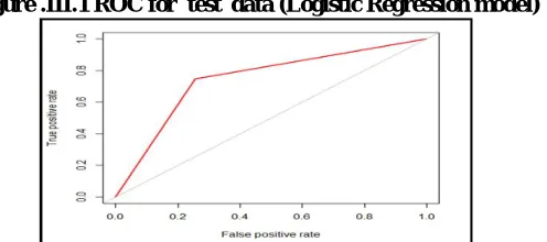
Area Under The Curve: The AUC obtained for the development data for the logistic regression model is 0.761. The AUC obtained for the test data is 0.736.
Figure .III.1 ROC for test data (Logistic Regression model)
Since the AUC value obtained for the logistic regression model is 0.736 we try to improve the model performance by applying Decision Tree which is discussed in Section III.2
III.2 DECISION TREE
Figure III.2 Decision tree from CART model
From the above Figure III.2 it can be seen that the first split happened on the basis of “ CustServ_Calls”. Further splits happened on the basis of “Day_Mins”, “Eve_Mins”, “Intl_Plan”, “Int_Calls” and “”Vmail_Message”. Having found the significant independent variables we will now evaluate the fit of the CART model through a Classification Table.
Accuracy Measures: The classification table for the CART model on the test data is given below:
Table III.4:Classification table(CART)
Predicted
Observed No Churn Churn
No Churn 759 89
Churn 25 126
From the above classification Table III.4 the accuracy of the CART model fitted on the test data is 0.885, that is, 88.5% of the total number of predictions are correct. We make use of classification Table 3.4 to visualize the performance of the CART model by the ROC curve and summarize its performance in a single number by computing the AUC.
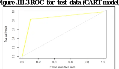
Area Under The Curve: The AUC obtained for the development data for the CART model is 0.863. The AUC obtained for the test data is 0.865.
Figure .III.3 ROC for test data (CART model)
III.3 RANDOM FOREST
The relative importance of the independent variables based on the Mean Decrease Gini Index have been obtained by applying the random forest model to the customer churn data. We have listed the independent variables based on Mean Decrease Gini below.
Table III.5: Variable importance measures from random forest model.
Variable Mean Decrease Gini
Day_Mins 75.36329
Day_Charge 74.51449
CustServ_Calls 67.49087
Intl_Plan 49.71943
Eve_Mins 39.72101
Eve_Charge 37.7947
Intl_Calls 28.9858
Intl_Charge 24.72174
Intl_Mins 24.44756
Night_Mins 21.89088
Night_Charge 21.30365
Vmail_Message 20.32958
Day_Calls 18.90698
Night_Calls 17.845
Account_Length 17.7104
Eve_Calls 16.22263
Vmail_Plan 13.53145
In a similar fashion, an importance plot also has been obtained. The variable importance plot from the Random Forest Model is shown below:
Figure .III.4 Variable importance plot of variables in the model.
Clearly the most important factor causing churn is total daytime minutes. The number of calls to customer care, total international minutes, international plan and Eve_Mins have all featured as prominent predictors of churn. The duration of account with the company has little effect on churn. We will now evaluate the fit of the Random Forest model through a Classification Table.
Accuracy Measures: The Classification table for Random forest on test data is given below
Table III.6:Classification table(Random Forest)
Predicted
Observed No Churn Churn
No Churn 725 123
From the above classification Table 3.6 the accuracy of the Random Forest model fitted on the test data is 0.856, that is, 85.6% of the total number of predictions are correct. We make use of classification Table 3.6 to visualize the performance of the Random Forest model by the ROC curve and summarize its performance in a single number by computing the AUC.
Area Under The Curve:The AUC obtained for the development data for the random forest model is 0.866. The AUC
obtained for the test data is 0.861.
Figure .III.5 ROC for test data(Random Forest Model)
Since the AUC value obtained for the Random Forest model is 0.861 we try to improve the prediction accuracy by applying Gradient Boosting which is discussed in Section III.4
III.4 GRADIENT BOOSTING
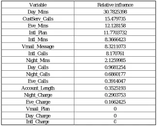
An ensemble model, Gradient Boosted trees also have been applied on the train data. While modeling, the relative influence for each of the variables has been calculated and are reported in the Table 3.7
Table III.7: Relative influence for each variable from Gradient Boost
Variable Relative influence
Day_Mins 30.7825398
CustServ_Calls 15.479735
Eve_Mins 12.128158
Intl_Plan 11.7703732
Intl_Mins 8.3666423
Vmail_Message 8.3211073
Intl_Calls 8.170761
Night_Mins 2.1259985
Day_Calls 0.9681254
Night_Calls 0.6860177
Eve_Calls 0.3914047
Account_Length 0.3525193
Night_Charge 0.2903753
Eve_Charge 0.1662425
Vmail_Plan 0
Day_Charge 0
It can be seen from Table III.7 that among the 17 predictors, 14 had non-zero influence. The most important among those predictors with high relative influence are Day_Mins, CustServ_Calls, Eve_Mins, Intl_Plan and Intl_Mins.
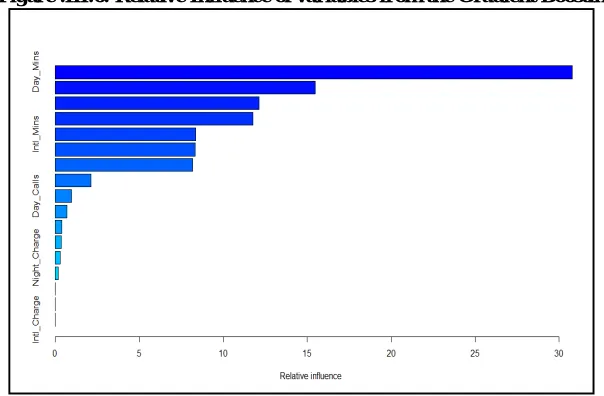
An importance plot has also been obtained. The variable importance plot from the Gradient Boosting Model is shown below:
Figure .III.6: Relative Influence of variables from the Gradient Boosting model.
From Figure .6 it can be observed that the most important factors causing churn are Day_Mins,
CustServ_Calls, Eve_Mins, Intl_Plan and Intl_Mins. We will now evaluate the fit of the Gradient Boosting model through a Classification Table.
Accuracy Measures: The Classification table for Gradient Boosting model on test data is given below
Table III.8: Classification table(Gradient Boosting)
Predicted
Observed No Churn Churn
No Churn 742 106
Churn 20 131
From the above classification Table 3.8 the accuracy of the Gradient Boosting model fitted on the test data is 0.873, that is, 87.3% of the total number of predictions are correct. We make use of classification Table 3.8 to visualize the performance of the Gradient Boosting model by the ROC curve and summarize its performance in a single number by computing the AUC.
Area Under The Curve:The AUC obtained for the development data for the Gradient Boosting model is 0.913 .The
Figure .III.7 ROC for test data(Gradient boosting)
III.5 COMPARISON OF PREDICTIVE MODELS
On the comparison of the AUC values of the test data, gradient boosting and decision trees seem to have good predictive power. From all the variable importance plots, it can be seen that tree based models i.e., CART, Random Forest and Gradient Boosting tend to give similar set of important independent variables. The most important independent variables can be observed to be :Day_Mins, CustServ_Calls,Intl_Plan and Eve_Mins.
IV. CONCLUSION
Based on all the results, the following recommendations are made. There is a strong correlation between higher total day minutes and churn. Almost half the customers with international plan end up switching to other providers. This could be due to a variety of factors. The voice mail plan seems to be popular with the customers. But not ‘enough’ customers seem to have opted for it. Customer’s account duration doesn’t seem to affect churn.
ACKNOWLEDGEMENT
The authors thank Mr Kannedari Siva Naga Raju, Research Scholar, Department of Statistics, Loyola College, Chennai-34 for his help and suggestions towards the article.
REFERENCES
1. Dr. M.Balasubramanian , M.Selvarani ;2014. “Churn Prediction In Mobile Telecom System Using Data Mining Techniques.”
2. Hangxia Ma, Min Qin, Jianxia Wang. (2009), “Analysis of the Business Customer Churn Based on Decision Tree Method”, The Ninth International Conference on Control and Automation, Guangzhou, China.
3. https://www.knime.org/knime-applications/churn-prediction
4. Manpreet Kaur, Dr. Prerna Mahajan;2015. “Churn Prediction in Telecom Industry Using R.” 5. M. Berry and G. Linoff. “Mastering Data Mining.” John Wiley and Sons, New York, USA, 2000.