An efficient procedure for the study of inhomogeneous liquids

PLEASE SCROLL DOWN FOR ARTICLE

On: 26 May 2009

Access details: Access Details: [subscription number 783677828] Publisher Taylor & Francis

Informa Ltd Registered in England and Wales Registered Number: 1072954 Registered office: Mortimer House, 37-41 Mortimer Street, London W1T 3JH, UK

Molecular Physics

Publication details, including instructions for authors and subscription information: http://www.informaworld.com/smpp/title~content=t713395160

An efficient procedure for the study of inhomogeneous liquids

a Department of Physics, North Carolina State University, Raleigh, NC 27695-8202, USA

First Published:February2009

To cite this Article Lado, F.(2009)'An efficient procedure for the study of inhomogeneous liquids',Molecular Physics,107:4,301 — 308 To link to this Article: DOI: 10.1080/00268970802603531

URL: http://dx.doi.org/10.1080/00268970802603531

Full terms and conditions of use: http://www.informaworld.com/terms-and-conditions-of-access.pdf This article may be used for research, teaching and private study purposes. Any substantial or systematic reproduction, re-distribution, re-selling, loan or sub-licensing, systematic supply or distribution in any form to anyone is expressly forbidden.

INVITED ARTICLE

An efficient procedure for the study of inhomogeneous liquids

F. Lado*

Department of Physics, North Carolina State University, Raleigh, NC 27695-8202, USA

(Received 20 October 2008; final version received 31 October 2008)

A complete description of an inhomogeneous fluid requires knowing not only its density(r) at any pointrin space, but also its pair distribution functiong(r1,r2). These can be found from coupled integral equations, but

even in cases with homogeneity in two of the three dimensions, such solutions in direct space are cumbersome enough to have earned the task a reputation as ‘computationally intensive’. Here we propose using purpose-built basis functions that are orthogonal with weight function(r) to expedite the work. We find that these not only produce a satisfying simplification of the formalism, but also reduce the computing effort needed to something on the order of 1% of that of the earlier calculations in direct space.

Keywords: inhomogeneous liquids; integral equations; Ornstein–Zernike equation; special orthogonal polynomials

1. Introduction

A complete description of an inhomogeneous fluid requires knowing not only its density(r) at any pointr in space, but also its pair distribution functiong(r1,r2)

describing the spatial correlation of two fluid particles at locations r1and r2. By the definition of

inhomoge-neous, this latter quantity is no longer just a function of

r12¼ jr1r2j and therein lies the special challenge of

solving Ornstein–Zernike (OZ) type integral equations for such systems. In many cases, the symmetry of a specific system will allow the general inhomogeneous OZ equation [1],

hðr1,r2Þ ¼cðr1,r2Þ þ Z

dr3hðr1,r3Þðr3Þcðr3,r2Þ, ð1Þ

to be partially deconvoluted using an integral transform, leaving a final one-dimensional integral unevaluated. (Here h(r1,r2)¼g(r1,r2)1 is the

inho-mogeneous pair correlation function and c(r1,r2) the

inhomogeneous direct correlation function effectively defined by the OZ equation.) Written in discrete form on a finite grid with summation replacing integration, this final equation for the transforms can then be interpreted as a matrix problem in direct space and solved accordingly. This usually entails a large number of spatial grid points and so the inhomogeneous liquid problem has acquired a reputation as computationally intensive (by integral equation standards, leaving aside simulation). In this note, for the Festschrift on the occasion of Jean-Jacques Weis’ retirement, we describe

how the remaining integral can also be analytically evaluated and the OZ equation reduced to an algebraic relation among expansion coefficients alone, just as for homogeneous molecular liquids, with an attendant sharp reduction in computing effort. This simplifica-tion is accomplished by the construcsimplifica-tion of tailored functions designed to be orthogonal with weight function(r).

The inhomogeneous OZ equation, coupled with an exact relation between the one-body and two-body functions (described below), was first solved for fluids in contact with a single hard wall by Sokolowski [2,3] and by Plischke and Henderson [4,5]. Liquids between two parallel walls (a planar slit) have been extensively and elegantly studied by Kjellander and Sarman [6–9]. These works all use a Hankel transform to eliminate two of the three integrals in the inhomogeneous OZ equation. Attard [10] has shown how the two angular integrals can be eliminated using a Legendre transformation for fluids with spherical inhomogene-ity. A clever application is then created by letting the spherical inhomogeneity arise from a fluid particle fixed at the origin of coordinates, so that an n-body distribution function in the inhomogeneous liquid becomes an (nþ1)-body distribution function in the original homogeneous system. Familiar approxima-tions now made at the nominal two-body level produce far better results [11–14] than when made at the conventional two-body level in a homogeneous formulation.

*Email: [email protected]

ISSN 0026–8976 print/ISSN 1362–3028 online ß2009 Taylor & Francis

DOI: 10.1080/00268970802603531 http://www.informaworld.com

In the next section, we describe a procedure that eliminates the surviving one-dimensional integral that complicates the task in the works cited above and finally converts the OZ equation into a purely alge-braic expression for the expansion coefficients alone. For specificity, we use the language of a planar slit; revising the notation for other geometries is straight-forward. Applications of the procedure are left to later works.

2. Reducing the OZ equation to algebra

A planar slit of width L is allowed to have indefinite wall extent so no boundary conditions are needed in the plane of the walls. The inhomogeneity then occurs perpendicular to the wall planes, which we denote conventionally as the zdirection. The density is now a one-dimensional function, (z), and pair functions such as h(r1,r2) can be described using coordinates

R12[(x1x2)2þ(y1y2)2]1/2, z1, and z2: thus,

h(r1,r2)¼h(R12,z1,z2), etc. The OZ equation now

reads

hðR12,z1,z2Þ ¼cðR12,z1,z2Þ þ Z L=2

L=2

dz3ðz3Þ

Z

dR3hðR13,z1,z3ÞcðR32,z3,z2Þ: ð2Þ

The first step in simplifying this equation is to use the homogeneity of the pair functions in the R plane to deconvolute it with a Hankel transform [2–9]:

^

hðK,z1,z2Þ ¼ Z

dRhðR,z1,z2ÞeiKR

¼2p

Z 1

0

dR R hðR,z1,z2ÞJ0ðKRÞ, ð3Þ

hðR,z1,z2Þ ¼ 1

ð2pÞ2 Z

dKh^ðK,z1,z2ÞeiKR

¼ 1

2p

Z 1

0

dK Kh^ðK,z1,z2ÞJ0ðKRÞ, ð4Þ

where J0(x) is the Bessel function of order zero.

We then obtain

^

hðK,z1,z2Þ ¼c^ðK,z1,z2Þ

þ ZL=2

L=2

dz3ðz3Þh^ðK,z1,z3Þc^ðK,z3,z2Þ,ð5Þ

with one remaining integral. This is the version of the OZ equation that all earlier papers have used. In practice, of course, the equation must be solved on a finite grid of points on the zaxis. If we use Nz

points, their spacing isz¼L/(Nz1) and the discrete

version is

^

hijðKÞ ¼c^ijðKÞ þ

X

Nz=2

k¼Nz=2

zkh^ikðKÞc^kjðKÞ, ð6Þ

wherej¼(zj),hˆij(K)¼hˆ(K,zi,zj), etc., with zj¼jz.

A more symmetric version of the equation can be obtained by multiplying through with (ij)1/2. In any

case, one now has a matrix equation that can be manipulated using standard matrix techniques. Since a large number of grid points is generally needed for an accurate numerical representation, the result is a calculation that is often deemed to be ‘computation-ally intensive’.

The usual remedy for this sort of problem is an expansion of thezdependence in orthogonal functions, with the critical expectation that far fewer expansion coefficients will be needed than grid points on the z

axis. Here that would ordinarily mean expansions in plane waves (using periodic boundary conditions),

EmðzÞ eimð2pz=LÞ

¼Tm½cosð2pz=LÞ þiVm½cosð2pz=LÞ, ð7Þ

wheremis a positive or negative integer. (For brevity, we will put

cosð2pz=LÞ ð8Þ

in the remainder of this work.) We recognize here

Tm()¼cos[m(2z/L)] as the type I Chebyshev

poly-nomial of order m and Vm()¼sin[m(2z/L)] the

associated Chebyshev function (not a polynomial) of orderm[15]. The familiar exponential functionsEm(z)

of course have the orthonormalization

1

L ZL=2

L=2

dz EmðzÞEm0ðzÞ ¼mm0, ð9Þ

where the asterisk denotes complex conjugate, for m,

m0_{positive or negative integers. But if we now put into}

Equation (5)

^

hðK,z1,z3Þ ¼ X1

m1,m3¼1 ^

Hm1m3ðKÞEm1ðz1ÞE

m3ðz3Þ, ð10Þ

and similarly forcˆ(K,z3,z2), the integral that turns up

is not Equation (9), but rather

1

L ZL=2

L=2

dzðzÞEmðzÞEm0ðzÞ,

and the invaluable property of orthogonality is lost. The essential proposal of this work is that one should simply replace the familiarEm(z) with specially

302 F. Lado

constructed basis functions Em(z) that are specifically

designed to be orthogonal with weight function (z). Preferring a dimensionless weight function, we define the mean density

¼1

L ZL=2

L=2

dzðzÞ, ð11Þ

and put ðzÞ ¼fðzÞ. Then the tailored orthogonal functions will be constructed to satisfy

1

L ZL=2

L=2

dz fðzÞEmðzÞEm0ðzÞ ¼_mm0, ð12Þ

again form,m0_{positive or negative integers, whilef(z)}

itself is normalized to unity,

1

L ZL=2

L=2

dz fðzÞ ¼1: ð13Þ

Now we may put

^

hðK,z1,z3Þ ¼ X1

m1,m3¼1 ^

hm1m3ðKÞEm1ðz1ÞE

m3ðz3Þ, ð14Þ

and similarly for cˆ(K,z3,z2), so that the OZ equation

finally becomes a relation among expansion coeffi-cients alone,

^

hm1m2ðKÞ ¼c^m1m2ðKÞ þL X1

m3¼1 ^

hm1m3ðKÞc^m3m2ðKÞ:

ð15Þ

We note that coefficients of all pair functions satisfy the symmetries

^

cm1m2ðKÞ ¼c^m2m1ðKÞ ¼c^m2m1ðKÞ ¼c^m1m2ðKÞ, ð16Þ

where m m. As usual, it is numerically preferable to eliminatehfrom the OZ equation and solve instead for the continuous ‘series’ function [16] s¼hc, for which we obtain

^

sm1m2ðKÞ ¼L X1

m3¼1

½s^m1m3ðKÞ þc^m1m3ðKÞc^m3m2ðKÞ:

ð17Þ

This is finally solved for the sˆm1m2(K); in matrix

notation,

^

SðKÞ ¼LC^ðKÞC^ðKÞ½ILC^ðKÞ1, ð18Þ

whereSˆ(K) andCˆ(K) are square matrices with elements

sˆm1m2(K) and cˆm1m2(K), respectively, and I is the unit

matrix. (Given the symmetries (16), only one-quarter

of the elements ofCˆ(K), etc., are unique.) The notable feature of Equation (18) is that it isidenticalto that of a homogeneous system. All of the inhomogeneity is built into the basis functions.

The construction of the tailored basis functions

Em(z),

EmðzÞ ¼ TmðÞ þiVmðÞ, ð19Þ

EmðzÞ ¼ EmðzÞ, ð20Þ

for m0, where Tm() and Vm() are the needed

generalized Chebyshev functions, is outlined in Section 4. We turn first to the relationship between

(z) and the pair functions.

3. Calculating the density profile

There are three exact equations that connect the one-body and two-body functions. Triezenberg and Zwanzig [17], Lovett et al. [18], and Wertheim [19] have shown that

d lnðz1Þ dz1

¼ dvextðz1Þ

dz1

ZL=2

L=2

dz2ðz2Þ

Z

dR2hðR12,z1,z2Þ

dvextðz2Þ dz2

¼ dvextðz2Þ

dz1

ZL=2

L=2

dz2ðz2Þh^ð0,z1,z2Þ

dvextðz2Þ

dz2

, ð21Þ

wherevext(z) is the external potential (here the walls of

the planar slit) and ¼(kBT) 1

the inverse Kelvin temperature, with kB Boltzmann’s constant.

Alternatively, passing through the OZ equation, this can be written as

d lnðz1Þ dz1

¼ dvextðz1Þ

dz1 þ

ZL=2

L=2

dz2

Z

dR2cðR12,z1,z2Þ dðz2Þ

dz2

¼ dvextðz1Þ

dz1 þ

ZL=2

L=2

dz2ðz2Þc^ð0,z1,z2Þ

d lnðz2Þ

dz2

: ð22Þ

The third exact equation is the first member of the Yvon–Born–Green hierarchy [20], which, for the sake of brevity, we will not examine here.

Becausef(z) is highly structured or even discontin-uous in the vicinity of the walls, we will solve for the

smoother and continuous combination f(z) exp[vext(z)]. We work first with Equation (21) and put

ln½fðzÞevextðzÞ _¼X 1

m¼0

AmTmðÞ, ð23Þ

^

hð0,z1,z2Þ ¼ X1

m1,m2¼1 ^

hm1m2ð0ÞEm1ðz1ÞE

m2ðz2Þ, ð24Þ

where we now seek to calculate the coefficients Am.

(Note that A0 is determined by normalization.)

We have for Equation (21),

X1

m¼1

Am dTmðÞ

dz ¼ X1

m1,m2¼1

h^m1m2ð0ÞEm1ðzÞ

ZL=2

L=2

dz0fðz0ÞE_m2ðz0Þdvextðz

0_Þ

dz0 : ð25Þ

Now multiply this equation by ði=LÞfðzÞE_m0ðzÞ and integrate over z. Then again invoking the orthonorm-ality integral, Equation (12), we arrive at the simple matrix equation

X1

m¼1

Dm0_mA_m¼H_m0: ð26Þ

Here we have defined

Dm0_m¼ 2

L ZL=2

0

dz fðzÞVm0ðÞ dTmðÞ

dz , ð27Þ

Hm0 ¼ L

X1

m¼1

½h^m0_mð0Þ h^_m0_mð0Þ 2

L

ZL=2

0

dz fðzÞVmðÞ

dvextðzÞ

dz , ð28Þ

and have used symmetry to simplify the integrals and the summation in Equation (28). A final matrix inversion in Equation (26) yields the coefficients Am

for the logarithm of the density profile.

Equation (22) works out in a similar fashion, with an extra matrix multiplication at the end. Since we havef(z) exp[vext(z)] as our objective, we first add and

subtract vext(z2) under the derivative d/dz2 on the

right-hand side of (22). This gives

d dz1

ln½fðz1Þevextðz1Þ

¼ ZL=2

L=2

dz2fðz2Þc^ð0,z1,z2Þ

d

dz2

ln½fðz2Þevextðz2Þ

ZL=2

L=2

dz2fðz2Þc^ð0,z1,z2Þ

dvextðz2Þ dz2

: ð29Þ

Again expanding functions as in Equations (23) and (24), we now have

X1

m¼1

Am dTmðÞ

dz ¼ X1

m¼1 X1

m1,m2¼1

c^m1m2ð0ÞAmEm1ðzÞ

ZL=2

L=2

dz0fðz0ÞE_m 2ðz

0_ÞdTmð0Þ

dz0

X

1

m1,m2¼1

c^m1m2ð0ÞEm1ðzÞ

ZL=2

L=2

dz0fðz0ÞE_m 2ðz

0_Þdvextðz0Þ

dz0 , ð30Þ

which we once more follow with a multiplication by

ði=LÞfðzÞE_m0ðzÞand integration overz. This yields

X1

m¼1 X1

m00_¼1

½m0_m00Lc^_m0_m00_ð0ÞD_m00_mA_m

¼ X

1

m00_¼1

c^m0_m00ð0Þ

ZL=2

L=2

dz fðzÞVm00ðÞ

dvextðzÞ dz : ð31Þ

Now put

Qm0_m¼

X1

m00_¼1

½m0_m00Lc^_m0_m00ð0ÞD_m00m, ð32Þ

Cm0¼ L

X1

m¼1

½c^m0_mð0Þ c^_m0_mð0Þ

2

L ZL=2

0

dz fðzÞVmðÞ

dvextðzÞ

dz , ð33Þ

so that the Am are again found by a simple matrix

inversion, now of

X1

m¼1

Qm0_mA_m¼C_m0: ð34Þ

Using the OZ Equation (15), one can show that Equations (26) and (34) are identical. Calculating the

Amseparately from both could be useful as an internal

numerical check.

4. Constructing the orthogonal functions

The familiar procedure for constructing a new set of orthogonal functions from a given complete set is the Gram–Schmidt method [15]. Thus, starting with the standard polynomials Tm()¼cos[m(2z/L)], the first

three (unnormalized) new polynomials of that are orthogonal with weight function f(z) can be explicitly written as

p0ðÞ ¼1, ð35Þ

304 F. Lado

p1ðÞ ¼T1ðÞ 1p0ðÞ, ð36Þ

p2ðÞ ¼T2ðÞ

3212þ1

2221þ1

p1ðÞ 2p0ðÞ,

ð37Þ

where the

j¼

2

L ZL=2

0

dz fðzÞTjðÞ ð38Þ

are modified moments of f(z). For computer calcula-tions, however, each new application of these succes-sive subtractions reduces the numerical precision, so that, in practice, this method becomes unusable beyond a small number of new polynomials.

Here we follow instead a robust approach described by Press and Teukolsky [21], based on works of Sack and Donovan [22] and Wheeler [23]. The monic version of the Chebyshev polynomials

Tm(),m()¼Tm()/2m1form40, have by

construc-tion a leading coefficient of unity. With1()0 and

0()1, they satisfy a standard recursion relation,

mþ1ðÞ ¼ ðTmÞmðÞ Tmm1ðÞ,

m¼0, 1, 2,. . ., ð39Þ

with T_m¼0 for all m and T₁ ¼1=2, T_m¼1=4 for

m41. The Press–Teukolsky algorithm then uses these monic coefficientsT

m,Tm along with the set

T j ¼

2

L Z L=2

0

dz fðzÞjðÞ, ð40Þ

or T_j ¼j=2j1 forj40, to recursively generate a new set of coefficientsamandbmsuch that, withP1()0

andP0()1, the monic polynomialsPm() generated

with these coefficients,

Pmþ1ðÞ ¼ ðamÞPmðÞ bmPm1ðÞ,

m¼0, 1, 2,. . ., ð41Þ

are orthogonal with weight function f(z). Thus to construct n polynomials Pm() for m¼1 through m¼n, we need the coefficients am, bm for m¼0

through m¼n1.

The key ingredient for this is the matrix [21]

kj¼ Pkjj

2

L Z L=2

0

dz fðzÞPkðÞjðÞ: ð42Þ

(Note thatkj¼0 fork4j.) It is clear that1,j¼0 for

alljand0j¼ Tj forj¼0,. . ., 2n1. Then the earlier recursions yield a recursion for thekj,

kj¼k1,jþ1þ ðjak1Þk1,j

þjk1,j1bk1k2,j, ð43Þ

for k¼1,. . .,n1 and j¼k,. . ., 2nk1. We set

a0¼0þ T1= T0 and b0¼0; then putting kþ1,k1¼0

andkþ1,k¼0 yields, respectively,

bk¼

kk

k1,k1

, ð44Þ

ak¼kþ

k,kþ1

kk

k1,k

k1,k1

, ð45Þ

for k¼1,. . .,n1, and the n monic polynomials

P1(),. . .,Pn() are determined by recursion,

Equation (41).

A final normalization yields the desired generalized Chebyshev polynomials,

T0ðÞ ¼1,

TmðÞ ¼

PmðÞ

½2hPmj Pmi1=2

, m¼1,. . .,n: ð46Þ

The algorithm further generates the roots1,2,. . .,n

ofTn()¼0 and the weightswjfor then-point Gauss–

Chebyshev quadrature,

2

L ZL=2

0

dz fðzÞFðÞ X

n

j¼1

wjFðjÞ: ð47Þ

The quadrature is exact if F() is a polynomial of degree less than or equal to 2n1, such as in Equation (27).

A similar procedure can now be followed for the generalizationUm() of type II Chebyshev polynomials Um() [15]. For this we need the corresponding monic

coefficients, U

m¼0 andUm¼1=4, for all m, and the modified moments

U j ¼

2

L ZL=2

0

dz fðzÞsin2ð2pz=LÞUjðÞ

2j : ð48Þ

It is easy to show that

U

0 ¼1=2 T 2, U

j ¼ Tj=4 Tjþ2, j40:

ð49Þ

The construction of theUm(), normalized to 1/2 with

weight functionf(z) sin2(2z/L), then follows precisely that of the Tm(), so we finally get the desired Vm()¼sin(2z/L)Um1().

By construction, then, these generalized Chebyshev functionsTm() andVm() satisfy

1

L Z L=2

L=2

dz fðzÞTmðÞTm0ðÞ ¼

1, m¼m0_¼0,

1=2, m¼m0_6¼0,

0, m6¼m0_, 8

> < > :

ð50Þ

1

L ZL=2

L=2

dz fðzÞVmðÞVm0ðÞ ¼

0, m¼m0_¼0,

1=2, m¼m0_6¼0,

0, m6¼m0_, 8

> < > :

ð51Þ

1

L ZL=2

L=2

dz fðzÞTmðÞVm0ðÞ ¼0, for allm,m0: ð52Þ

Collectively, Equations (50)–(52) give rise to the orthonormalization of Em(z) expressed in

Equation (12).

5. An illustration

In this section, we illustrate some practical details regarding the formal tailored polynomials discussed above. As noted earlier, actual applications will be left to later work.

For purposes of illustration we choose a system of hard spheres of diameterbetween parallel hard walls a distance Lapart [6,9]. The external potential is then

vextðzÞ ¼

0, jzj ðLÞ=2,

1, ðLÞ=25jzj L=2,

ð53Þ

so that the initial (non-interacting) density profile of the system is

fðzÞ ¼ L L H

L

2 þz

H L

2 z

, ð54Þ

whereH(x) is the Heaviside unit step function and the prefactor is chosen for normalization, Equation (13). In this case, we can calculate the needed T

j ¼

ð2=LÞR₀L=2 dz fðzÞjðÞanalytically. We obtain T

0 ¼1, ð55Þ

T j ¼

Lsinðjp=LÞ jpðLÞ

1 2

j1

, j40, ð56Þ

and the appropriate Tm[cos(2z/L)] are then

con-structed following the recipe in Section 4.

We have arbitrarily chosen L¼5 for these calculations and show in Figure 1 the first four special polynomials T1(),. . .,T4() generated for this case

(omitting the trivial T0()¼1). They are seen to be

quite changed from the original constant-amplitude Chebyshev form, Tm()¼cos[m(2z/L)]. Similarly,

the corresponding first four generalizations of

Vm()¼sin[m(2z/L)], V1(),. . .,V4(), seen in

Figure 2, also display variable amplitudes, though of course they still vanish at the end points. Note that the integral common to both Equation (28) and (33) picks

up the values of these latter functions at the cutoff,

z¼(L)/2:

2

L ZL=2

0

dz fðzÞVmðÞ

dvextðzÞ dz

¼ 2

L ZL=2

0

dz fðzÞevextðzÞ_V

mðÞ

devextðzÞ

dz

¼2 L

ZL=2

0

dz fðzÞevextðzÞ_V

mðÞ z

L

2

¼ 2

L Vm cos

L

L p

: ð57Þ

It is clear from the earlier sections that the proce-dure proposed here at least yields a satisfying simpli-fication of the formalismused to solve the prescribed equations for a full description of an inhomogeneous fluid. The practical question, however, is whether it

−4 −2 0 2 4 6 8

−2 −1 0 1 2

Tm (z)

z/s

Figure 1. Tailored orthogonal polynomials T1(), T2(), T3(), T4() generalizing the ChebyshevTm()¼cos[m(2z/

L)] constructed for the rectangular (ideal) density profile of Equation (54) for slit widthL¼5; herecos(2z/L).

−2 −1 0 1 2

−2 −1 0 1 2

z/s

Vm (z)

Figure 2. Tailored orthogonal functionsV1(), V2(),V3(), V4() generalizing the Chebyshev Vm()¼sin[m(2z/L)] constructed for the rectangular (ideal) density profile of Equation (54) for slit widthL¼5; herecos(2z/L).

306 F. Lado

also produces a significant reduction in computing time for these solutions, perhaps even putting such calculations on a par with those of homogeneous systems. This is essentially a question of how the number of coefficients, sayn, used in an expansion like (23) compares with the number of grid points, say Nz,

needed for an equally good representation of the same function directly on the z axis. In a real calculation, Equation (23) would be used to find ln{f(z)exp[vext(z)]} from the calculated Am. Here we

are going to turn that around, create a realistic model of a continuous density profile on the z grid, and see how many coefficientsAmare required to reproduce it.

For the modeled density profile we turn to the Percus–Yevick (PY) equation for hard spheres [20]. Specifically, we start with the continuous function

gHS(r) exp[vHS(r)] that the PY equation produces at

3¼0.8 with a grid interval r¼0.02, cut out the section fromr¼0.5 tor¼3.0, and call that the left half of our modeled density profile, f0(z) exp[vext(z)],

over the intervalz¼ 2.5toz¼2.5withz¼0.02. Then we simply fold that piece over to produce the symmetric right half; the result is shown in Figure 3. This continuous density profile is not a very familiar quantity. If, however, we now truncate this shape at

(L)/2 (that is, multiply by exp[vext(z)]), we get

the discontinuous density profilef0(z) seen in Figure 4.

This is indeed a familiar quantity. Specifically, it strongly resembles (by design) the density profile computed by Kjellander and Sarman [9] for a hard sphere fluid between hard walls at separation L¼5

and shown as their Figure 1(e). Thus, the data for Figure 3 will serve as our realistic test profile. It is based on Nz¼250 grid points; we then use

fourth-order interpolation to obtain the test density profile at the n points needed for the Gauss–Chebyshev quad-rature below.

Applying the expansion of (23) to our test profile, we have

ln½f0ðzÞevextðzÞ ¼ Xn1

m¼0

AmTmðÞ, ð58Þ

where we are still using the special polynomials Tm()

constructed for the f(z) of Equation (54) and sampled in Figure 1. Thus, multiplying this equation by (1/L)

f(z)Tk() and integrating over zproduces, fork40,

Ak¼ 2

L ZL=2

L=2

dz fðzÞln½f0ðzÞevextðzÞTkðÞ

¼2X

n

j¼1

wjln½f0ðzjÞevextðzjÞTkðjÞ, ð59Þ

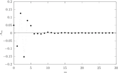
after invoking Equations (50) and (47). The quadrature is now evaluated for successive values ofk; the results are shown graphically as Am vs. m in Figure 5, for

which we have usedn¼30. It seems clear that, holding

n fixed at 30, fewer than the 30 coefficients Am

(numbered 0 through 29) seen in the figure would actually suffice in the expansion (58). In fact, we anticipate that the cutoff limits for single index expansions such as (23) or double index expansions such as (14) may be set at some integer nc that is

meaningfully smaller than the given n, which is kept larger to set the parameters for the Gauss–Chebyshev quadratures.

We conclude that the number nc of coefficients

needed in the tailored orthogonal functions procedure put forward in this work will be about an order of magnitude smaller than the number of grid pointsNz

needed for the direct space procedures used in earlier works. Since much of the numerical effort involves

0 2 4 6 8 10 12 14

−2 −1 0 1 2

f0

(z)e

b

vext(z)

z/s

Figure 3. Continuous test profilef0(z) exp[vext(z)] for hard

spheres between hard walls with a slit width L¼5, constructed using gHS(r) exp[vHS(r)] from the Percus–

Yevick equation for hard spheres at3¼0.8. See text.

0 0.5 1 1.5 2 2.5 3 3.5 4 4.5

−2 −1 0 1 2

f0

(z)

z/s

Figure 4. Discontinuous test profile f0(z) for hard spheres

between hard walls with a slit width L¼5 obtained by truncation of the form in Figure 3 atz¼ (L)/2.

matrix operations, of order N2

z in Equation (6) vs. n2c in Equation (15), we may reasonably conclude that solutions obtained using the tailored orthogonal functions will require on the order of 1% of the computational effort of those earlier works. That should make equations for inhomogeneous fluids as readily solvable as their more familiar homogeneous cousins.

References

[1] D. Henderson, in Fundamentals of Inhomogeneous Fluids, edited by D. Henderson (Dekker, New York, 1992), Chap. 4.

[2] S. Sokolowski, J. Chem. Phys.73, 3507 (1980). [3] S. Sokolowski, Mol. Phys.49, 1481 (1983).

[4] M. Plischke and D. Henderson, Proc. R. Soc. Lond. A

404, 323 (1986).

[5] M. Plischke and D. Henderson, J. Chem. Phys.84, 2846 (1986).

[6] R. Kjellander and S. Sarman, Chem. Phys. Lett. 149, 102 (1988).

[7] R. Kjellander and S. Sarman, Mol. Phys. 70, 215 (1990).

[8] R. Kjellander and S. Sarman, Mol. Phys.74, 665 (1991). [9] R. Kjellander and S. Sarman, J. Chem. Soc. Faraday

Trans.87, 1869 (1991).

[10] P. Attard, J. Chem. Phys.91, 3072 (1989). [11] P. Attard, J. Chem. Phys.91, 3083 (1989). [12] S.A. Egorov, J. Chem. Phys.112, 7138 (2000).

[13] E. Lomba, S. Jorge, and M. A´lvarez, Phys. Rev. E63, 011203 (2000).

[14] J.M. Brader, J. Chem. Phys.128, 104503 (2008). [15] G. Arfken, Mathematical Methods for Physicists

(Academic Press, Orlando, 1985).

[16] M.S. Green, J. Chem. Phys. 33, 1403 (1960); ibid. 39, 1367 (1963). Green classified the diagrams in the density expansion ofg(r) ev(r)by analogy with electric circuits as ‘series’, ‘parallel’, or ‘bridge’, the last because of the resemblance of the first diagram to a Wheatstone bridge. The ‘parallel’ terms can be summed in direct space and disappear. The name ‘series’ is nowadays seldom used but the ‘bridge’ name incongruously survives.

[17] D.G. Triezenberg and R. Zwanzig, Phys. Rev. Lett.28, 1183 (1972).

[18] R. Lovett, C.Y. Mou, and F.P. Buff, J. Chem. Phys.65, 570 (1976).

[19] M.S. Wertheim, J. Chem. Phys.65, 2377 (1976). [20] J.P. Hansen and I.R. McDonald, Theory of Simple

Liquids(Academic Press, London, 1986).

[21] W.H. Press and S.A. Teukolsky, Comp. Phys. 4, 423 (1990).

[22] R.A. Sack and A.F. Donovan, Num. Math. 18, 465 (1971/72).

[23] J.C. Wheeler, Rocky Mount. J. Math.4, 287 (1974). Figure 5. CoefficientsAmfor the expansion of Equation (58)

as a function of integerm.

308 F. Lado