Publisher: Institute for Operations Research and the Management Sciences (INFORMS) INFORMS is located in Maryland, USA
Stochastic Systems
Publication details, including instructions for authors and subscription information: http://pubsonline.informs.org
Randomized Assignment of Jobs to Servers in
Heterogeneous Clusters of Shared Servers for Low Delay
Arpan Mukhopadhyay, A. Karthik, Ravi R. Mazumdar
To cite this article:
Arpan Mukhopadhyay, A. Karthik, Ravi R. Mazumdar (2016) Randomized Assignment of Jobs to Servers in Heterogeneous Clusters of Shared Servers for Low Delay. Stochastic Systems 6(1):90-131. https://doi.org/10.1287/15-SSY179
Full terms and conditions of use: https://pubsonline.informs.org/page/terms-and-conditions
This article may be used only for the purposes of research, teaching, and/or private study. Commercial use or systematic downloading (by robots or other automatic processes) is prohibited without explicit Publisher approval, unless otherwise noted. For more information, contact [email protected].
The Publisher does not warrant or guarantee the article’s accuracy, completeness, merchantability, fitness for a particular purpose, or non-infringement. Descriptions of, or references to, products or publications, or inclusion of an advertisement in this article, neither constitutes nor implies a guarantee, endorsement, or support of claims made of that product, publication, or service.
Copyright © 2016, The author(s)
Please scroll down for article—it is on subsequent pages
INFORMS is the largest professional society in the world for professionals in the fields of operations research, management science, and analytics.
2016, Vol. 6, No. 1, 90–131 DOI:10.1214/15-SSY179
RANDOMIZED ASSIGNMENT OF JOBS TO SERVERS IN HETEROGENEOUS CLUSTERS OF SHARED SERVERS
FOR LOW DELAY
By Arpan Mukhopadhyay, A. Karthik, and Ravi R. Mazumdar
University of Waterloo
We consider the problem of assignning jobs to servers in a multi-server system consisting ofN parallel processor sharing servers, cat-egorized intoM (N) different types according to their processing capacities or speeds. Jobs of random sizes arrive at the system ac-cording to a Poisson process with rateN λ. Upon each arrival, some servers of each type are sampled uniformly at random. The job is then assigned to one of the sampled servers based on their states. We propose two schemes, which differ in the metric for choosing the des-tination server for each arriving job. Our aim is to reduce the mean sojourn time of the jobs in the system.
It is shown that the proposed schemes achieve the maximal sta-bility region, without requiring the knowledge of the system param-eters. The performance of the system operating under the proposed schemes is analyzed in the limit asN → ∞. This gives rise to a mean field limit. The mean field is shown to have a unique, globally asymp-totically stable equilibrium point which approximates the stationary distribution of load at each server. Asymptotic independence among the servers is established using a notion ofintra-type exchangeability
which generalizes the usual notion of exchangeability. It is further shown that the tail distribution of server occupancies decays doubly exponentially for each server type. Numerical evidence shows that at high load the proposed schemes perform at least as well as other schemes that require more knowledge of the system parameters.
1. Introduction. Consider a stream of jobs arriving at a multi-server system consisting of a large number of parallel processor sharing servers. The servers are categorized into different types or clusters according to their processing capabilities. Each job, upon arrival, is assigned to a server where it completes its service and leaves the system. The objective is to design job assignment schemes that reduce the average sojourn, or response, time of jobs in the system.
Received February 2015.
MSC 2010 subject classifications:Primary 60K35; secondary 60K25, 90B15.
Keywords and phrases:Processor sharing, power-of-two, mean field, asymptotic inde-pendence, stability, propagation of chaos.
1.1. Motivation. The problem of job assignment is central in multi-server resource sharing systems that process delay sensitive web requests. Exam-ples include data centers and web server farms running applications such as online search, social networking etc. In these systems, a small increase in the average response time of requests may cause significant loss of revenue and users [21]. Therefore, it is critical to reduce the average response time of jobs in such systems.
Reduction in the average response time can be achieved by assigning new arrivals to less congested servers [25,10,26] in the system. However, in sys-tems, where the number of servers is large, obtaining state information of all the servers may incur significant overhead and delay. For such systems, randomized job assignment schemes, in which each assignment decision is made based on comparing the states of a small random subset of d (≥ 2) servers, are promising solutions. For systems with identical servers (homo-geneous), such randomized schemes have been shown [24,14,9] to result in an exponential reduction in mean response time of jobs as compared to state independent schemes, in which job assignments are made independently of the states of the servers. This implies that for large homogeneous systems, a small, randomly chosen subset of servers is representative of the distribution of load in the overall system.
In this paper, we consider heterogeneous systems where servers are grouped into different types or clusters, often geographically separated, based on their capacities. For such systems, sampling servers without taking into account the different server types may lead to instability [18,17]. We therefore con-sider randomized job assignment schemes, in which a small random subset of servers is sampled from each server type. The least loaded servers of each type are then compared based on some metric. The job is then assigned to the “best” server that is likely to yield the least delay. We consider processor sharing (PS) as the service discipline in this paper since it closely approxi-mates round-robin discipline with small granularity [20] usually employed in server farms. Moreover, processor sharing discipline has the desirable prop-erty of being insensitive to job length distribution type [12].
1.2. Related literature. Randomized job assignment schemes have been primarily studied in the literature for a system consisting ofN identical first come first serve (FCFS) servers, which is also referred to as the supermarket model. Most studies consider the so called SQ(d) scheme in which each job is assigned to the shortest ofdrandomly chosen queues.
same result using an extension of Kurtz’s theorem [7]. In [23], a coupling argument was used to show that larger values ofdresult in more even distri-bution of loads among the servers. Chaoticity on path space (or asymptotic independence among queue length processes) was established in [9] using empirical measures on the path space of the underlying Markov processes. Results of [24] were generalized to the case of open Jackson networks in [13]. Recently, in [4], the SQ(d) scheme was analyzed under more general ser-vice disciplines and serser-vice time distributions. It was shown that in the case of FCFS discipline and power-law service time distribution, the equilibrium queue sizes decay doubly exponentially, exponentially, or just polynomially, depending on the power-law exponent and the number of choices, d. The stability of more general randomized schemes for non-idling service disci-plines was analyzed in [3], which derived a sufficient condition under which such networks are stable. Asymptotic independence of servers in equilibrium was proposed in [5] under local service disciplines and general service time distributions. However, the result was proved only for FCFS service disci-pline and service time distributions having decreasing hazard rate (DHR) functions.
The tradeoff between sampling cost of servers and the expected sojourn time seen by a customer in the supermarket model was studied under a game theoretic framework in [28]. It was shown that for arrival rates within the stability region of the network, a symmetric Nash equilibrium for identical customers exists in which each customer chooses a fixed number of queues to sample. Randomized schemes similar to the SQ(d) scheme were also used in [19] for cache eviction based on cache hit rate.
randomized job assignment in loss systems where the analysis is different due to finiteness of the state space.
1.3. Main results. This paper focuses on the design and analysis of ran-domized job assignment schemes which achieve the maximal stability region for heterogeneous processor sharing systems without requiring the knowl-edge of system parameters and yet yield smaller delays than randomized state independent schemes. To this end, we propose two schemes in which random subsets of servers are sampled from each type at each arrival instant. The job is then assigned to the “best” server among all the sampled servers. The metric for choosing the best server distinguishes the two schemes.
The schemes can be implemented as follows: A central dispatcher, upon arrival of a new job, first requests local routers at each cluster of servers having the same speed to send the index of a server from its corresponding cluster. The local router then samples some servers from the corresponding cluster uniformly at random and sends the index of the least loaded sampled server to the central dispatcher. The central dispatcher finally compares the states of the servers whose indices it has received and selects “best” server as the final destination of the arriving job.
In the first scheme, the “best” server is selected simply based on the number of jobs in the progress whereas in the second scheme, the sampled server offering the maximum processing rate is taken to be the “best” server. We note that, in the both the schemes, servers of all types are compared to make job assignment decisions. We show that due to such sampling, the proposed schemes achieve the maximum possible stability region.
We analyze the performance of the proposed schemes in the limit as the system sizeN → ∞ using the mean field approach. Our contributions are the following.
• We establish that the underlying Markov process describing the system converges to a mean field using the theory of operator semigroup for Markov processes as in [13,2].
• The mean field is shown to have a unique, globally asymptotically stable equilibrium point in the space of empirical tail measures hav-ing finite first moment. Our proof differs significantly from the earlier works since in the heterogeneous case closed form expression for the equilibrium point cannot be obtained.
• Propagation of chaos or asymptotic independence among servers is shown to hold at each finite time and also at the equilibrium. To show this, we generalize the standard notion of exchangeability to the notion ofintra-type exchangeability to deal with random variables having different distributions.
• The stationary tail distribution of server occupancies is shown to de-cay doubly exponentially in the limiting system. We devise an indirect method to show this, since, unlike the homogeneous case, closed form solutions of the stationary distribution cannot be obtained in the het-erogeneous scenario.
Numerical comparison of the proposed schemes with existing schemes shows the superiority of the proposed schemes in terms of reducing the mean response time of jobs while requiring no knowledge of the system parameters.
1.4. Organization. The rest of the paper is organized as follows. In Sec-tion2, we describe the system model, the proposed job assignment schemes and our notations. We then analyze the proposed schemes in Sections 3,4, and 5. In Section 6, numerical results are presented that compare the pro-posed schemes with other existing schemes to determine their efficacy. Fi-nally, we conclude the paper in Section7 with a summary and a discussion on future work.
2. Model and notations. We consider a multi-server system consist-ing ofN parallel processor sharing (PS) servers. The capacity,C (bits/sec), of a server is defined as the time rate at which it processes a single job present in it. If there areq(t) jobs present at a server of capacityC at time
t, then the instantaneous rate at which each job is processed in the server is given byC/q(t). Depending on their capacities, the servers in the system are categorized into M ( N) types. Define J = {1,2, . . . , M} to be the index set of server types. The capacity of typejservers is denoted byCj, for
j∈ J, and we assume, without loss of generality, that the server capacities are ordered in the following way:
(2.1) C1 ≤C2≤. . .≤CM.
Further, for eachj ∈ J, we denote the proportion of type j servers in the system byγj (0≤γj ≤1). Clearly,
M
j=1γj = 1.
Fig 1. System consisting ofN parallel processor sharing (PS) servers, categorized intoM types. There areγjN servers of typej, each of which has a capacity or rateCj. Arrivals occur according to a Poisson process with rateN λ. For each arrival,dj servers of typej are sampled. The arrival is finally sent to to one of the sampled servers for processing.
of jobs in progress at each server does not depend on the type of job length distribution (as long as the mean of the distribution remains unchanged) due to the insensitivity of the processor sharing discipline. The inter-arrival times and the job lengths are assumed to be independent of each other. Upon arrival, a job is assigned to one of the N servers where the job stays till the completion of its service after which it leaves the system. The model is illustrated in Figure 1. We consider the following two job assignment schemes.
2.1. Scheme 1. In this scheme, upon arrival of a job,dj servers of typej
are sampled uniformly at random from the set ofN γj servers of typej, for
each j∈ J. Note that this sampling is done at the cluster of type j servers by a local router.
Let
q(Nj,1), qN(j,2), . . . , qN(j,dj)
denote the vector of occupancies of the dj
sampled servers of typej. For each typej ∈ J, a sampled server with index
kj is chosen for further comparison where kj is given by
(2.2) kj = arg min
1≤r≤dj
q(Nj,r)
.
[image:7.612.185.425.114.310.2]uniformly at random from the tied servers of that type. The occupancy information of the server corresponding tokjis sent to the central dispatcher.
Using this information from each of the clusters j ∈ J the arriving job is assigned by the dispatcher to the typei sampled server having index ki
where
(2.3) i= arg min
1≤j≤M
q(j,kj) N
.
Ties across server types are broken by choosing the server type having the highest capacity among the tied servers. Thus, in this scheme, each arrival is assigned to the server having the least instantaneous occupancy among the subset of randomly selected servers.
2.2. Scheme 2. As in Scheme 1, upon arrival of a job, a random subset of dj servers of type j is chosen uniformly, for eachj∈ J. Then from each
type j ∈ J, a server with index kj is chosen according to (2.2) for further
comparison across different server types. The arriving job is finally assigned to the typeisampled server having indexki if
(2.4) i= arg max
1≤j≤M
Cj/q
(j,kj) N
.
Note that the quantity Cj/q(Nj,kj) denotes the processing rate per
unfin-ished job at the sampled typej server with index kj. Thus, in this scheme,
an arrival is assigned to the server that provides the highest processing rate per job among the sampled set of servers. Ties are broken in the same way as described in Scheme 1.
It is clear that Scheme 2 differs from Scheme 1 only in the criterion for server selection. In Scheme 1, server selection is done based only on the in-stantaneous occupancies of the sampled servers, whereas in Scheme 2 server capacities are also taken into account in the selection criterion. Note that in the heterogeneous scenario a server with higher occupancy can still pro-vide a higher processing rate than a server with lower occupancy. Therefore, Scheme 2 provides a finer metric for server selection.
2.3. Notations. We define the following real sequence spaces:
¯
U(j)
N ={{gn}n∈Z+ :g0= 1, gn≥gn+1≥0, N γjgn∈N∀n∈Z+},
(2.5) ¯
U ={{gn}n∈Z+ :g0= 1, gn≥gn+1≥0 ∀n∈Z+},
(2.6)
U ={{gn}n∈Z+ :g0= 1, gn≥gn+1≥0 ∀n∈Z+, ∞
n=0
gn<∞}.
Letj∈J U¯N(j), ¯UM, and UM denote the Cartesian products of ¯UN(j), ¯U, and
U, respectively, over j∈ J. An element u =
u(nj), j ∈ J, n∈Z+
belongs
toj∈JU¯N(j), ¯UM, orUM if for eachj∈ J, the sequenceu(j) n
n∈Z+
belongs
to ¯UN(j), ¯U, orU, respectively. Foru,w∈U¯M we define the following distance metric
(2.8) u−w = sup
j∈J
sup
n∈Z+
u(nj)−w(nj)
n+ 1
.
It can be easily verified that under the metric defined in (2.8), the space ¯UM is compact (and hence complete and separable). Further, for any k ∈ Z+
and i, j∈ J, we define
kij =
Cj
Ci
k + 1,
(2.9)
kij =
Cj
Ci
k
,
(2.10)
wherex denotes the greatest integer not exceedingxand xdenotes the smallest integer greater than or equal tox.
Let (H,H, μH) be a measure space and f :H → R be a μH-integrable
function. We define duality brackets as f, μH =
f dμH. We denote the
weak convergence (convergence in distribution) of a sequence of probability measures Pn (random variables Xn) to a probability measure P (random
variableX) byPn⇒P (Xn⇒X).
3. Stability analysis. In this section, we derive the sufficient condition for the system to ne stable, i.e., to have a finite expected number of jobs at all times under Scheme 1 and Scheme 2.
To formally state our results, we define the process
(3.1) xN(t) =
x(N,nj) (t), j∈ J, n∈Z+
fort≥0,
where x(N,nj) (t) denotes the fraction of type j servers having at least n un-finished jobs at time t. Thus,
x(N,nj) (t), n∈Z+
denotes the empirical tail distribution of occupancy of type j servers at time t. Clearly, xN(t) is a
Markov process in the state spacej∈JU¯N(j).
We now find the set of arrival rates for which the Markov processxN(·) ispositive recurrent orstable.
(3.2) λ < μ
j∈J
γjCj.
Furthermore, for λ > μj∈J γjCj the system is unstable under any job assignment scheme.
Proof. We provide a proof via coupling argument. Consider a modified
scheme in which, upon arrival of each job, one server is chosen from each type uniformly at random (i.e., dj = 1 for all j ∈ J). The job is then
routed to the sampled server of type j with probability γjCj
i∈JγiCi for each
j∈ J. A simple coupling argument, similar to the one discussed in the proof of Theorem 3 of [13], shows that the system operating under the modified scheme always has higher number of unfinished jobs than that operating under Scheme 1 or Scheme 2.
Now the system operating under the modified scheme is stable if the arrival rate to any server is less than the service rate at the server. Clearly, the rate of arrival of jobs at a type j server under the modified scheme is
N λ× N γ1
j × γjCj
i∈JγiCi = λCj
i∈JγiCi. The service rate of a type j server is
μCj. Hence, condition (3.2), guarantees that the arrival rate is smaller than
the service rate for each type of servers. This implies that under (3.2) the system is stable under the modified scheme. Due to the coupling argument described above it also implies that under (3.2) the system is stable under Scheme 1 and Scheme 2.
As discussed in [3], forλ > μj∈JγjCj, the system under consideration
is unstable under any job assignment policy.
Thus, from Theorem3.1we conclude that Scheme 1 and Scheme 2 achieve the maximal stability region given by (3.2).
4. Mean field analysis. We now analyze the time evolution of the process xN(·) under Scheme 1 and Scheme 2. Its exact characterization is difficult since under both the schemes, arrivals at a given server depend on the states of other servers. However, it is possible to analyze the system in the limit as the system size N → ∞. We show that the process xN(·) weakly converges to a deterministic processu(·) asN → ∞. We also show that the steady state behavior of the processxN(·) can be approximated by
the equilibrium point of the processu(·) for large values ofN.
Theorem4.1. If xN(0) converges in distribution to some constant g∈
¯
UM as N → ∞, then the process {x
N(t)}t≥0 converges in distribution to
a process {u(t)}t≥0, lying in the space U¯M as N → ∞. For Scheme 1, the process u(t) is given by the solution of the following system of differential equations
u(0) =g,
(4.1)
˙
u(t) =l(u(t)),
(4.2)
where the mappingl: ¯UM →RZ+M is given by
l(0j)(u) = 0, for j ∈ J,
(4.3)
l(kj)(u) = λ
γj
u(kj−)1
dj
−u(kj)
djj−1
i=1
u(ki−)1
di M
i=j+1
u(ki)
di
(4.4)
−μCj
u(kj)−u(kj+1)
, for k≥1, j ∈ J.
For Scheme 2, the processu(t) is given by the solution of
u(0) =g,
(4.5)
˙
u(t) =˜l(u(t)),
(4.6)
where the mapping˜l: ¯UM →RZ+M is given by
˜l(j)
0 (u) = 0, for j∈ J,
(4.7)
˜l(j)
k (u) =
λ γj
u(kj−)1
dj
−u(kj)
djj−1
i=1
u(ik)−1ji
di
(4.8)
× M
i=j+1
u(ik)−1 ji
di
−μCj
u(kj)−u(kj+1)
, for k≥1, j∈ J.
The processu(·), defined in the theorem above, is referred to as themean field limit of the system. To emphasize the dependence of the process u(·) on the initial point u(0) =g, we will often denote u(t) by u(t,g).
Remark 4.1. We note that Theorem 4.1 implies that if xN(0) ⇒ g ∈
¯
UM asN → ∞, then the following weaker convergence results also hold:
1. For eacht≥0,xN(t)⇒u(t,g) asN → ∞.
3. For eacht≥0,j∈ J, andk∈Z+,E
x(N,kj) (t)
→u(kj)(t,g) asN → ∞.
The last assertion follows from the first since x(N,kj) (t) is bounded for each
N, j, k, t.
We first note that Theorem4.1implicitly assumes that the ordinary differ-ential systems (4.1)–(4.2) and (4.5)–(4.6) have unique solutions in the space
¯
UM. In the following proposition, we show that this is indeed the case.
Proposition 4.1. If g ∈ U¯M, then each of the systems (4.1)–(4.2) and (4.5)–(4.6) has a unique solution u(t,g)∈U¯M, for allt≥0.
Proof. The proof is given in Appendix A.
We will prove Theorem 4.1 using the theory of semigroup operators of Markov processes as in [24, 13, 2]. Some of the key definitions and results which we use in this topic are given in Appendix E. For more details the reader is referred to [7]. First, we recall the following:
• The operator semigroup{TN(t)}t≥0 corresponding to the Markov
pro-cessxN(·) acting on continuous functionsf : M
j=1U¯ (j)
N →Ris defined
as
TN(t)f(x) =E[f(xN(t))|xN(0) =x] ∀t≥0,x∈
j∈J
¯
U(j)
N .
• For the deterministic process {u(t)}t≥0, the transition semigroup
{T(t)}t≥0 acting on continuous functionsf : ¯UM →Ris defined as
T(t)f(x) =f(u(t,x)) ∀t≥0,x∈U¯M.
In the next proposition, we show that{TN(t)}t≥0 converges to{T(t)}t≥0
uniformly on bounded intervals. The above fact in conjunction with Theorem 2.11 of Chapter 4 of [7] proves Theorem4.1.
Proposition 4.2. For both Scheme 1 and Scheme 2, and for any con-tinuous functionf : ¯UM →R and t≥0,
(4.9) lim
N→∞ sup
g∈j∈JU¯N(j)
|TN(t)f(g)−f(u(t,g))|= 0
and the convergence is uniform in twithin any bounded interval.
4.2. Properties of the mean field. In this section, we characterize some important properties of the mean field. In particular, we show that, under the stability condition (3.2), both (4.1)–(4.2) and (4.5)–(4.6) have unique equilibrium points inUM. Further, we show that the equilibrium points are globally asymptotically stable for both systems.
Let P, ˜P denote the equilibrium points of (4.1)–(4.2) and (4.5)–(4.6), respectively. In other words,Pand ˜Psatisfyl(P) =0 and˜l(P˜) =0. Hence, for allk∈Z+ and j ∈ J the following must hold
(4.10) Pk(j+1) −Pk(+2j) = Δj
Pk(j)
dj
−Pk(j+1)
dj
× j−1
i=1
Pk(i)
di M
i=j+1
Pk(i+1)
di
,
(4.11) P˜k(j+1) −P˜k(+2j) = Δj
˜
Pk(j)
dj
−P˜(j)
k+1
dj
× j−1
i=1
˜
P(ki)ji
di M
i=j+1
˜
P(ki) ji
di
,
where Δj = μγλjCj for each j ∈ J. Note that by definition we have P0(j) =
˜
P0(j) = 1 for allj∈ J. The next proposition reveals an important property of the equilibrium points P and ˜P. To state it we first need the following definition.
Definition 4.1. A real sequence{zn}
n≥1 is said to decrease doubly
ex-ponentially if and only if there exist positive constantsL, ω <1, θ >1, and
κ such that zn≤κωθ n
for all n≥L.
Hence, if a sequence {zn}n≥1 decays doubly exponentially, then it is
summable, i.e., ∞n=1zn<∞.
Proposition4.3. Assume that for eachj∈ J,P(j) k ,P˜
(j)
k ↓0ask→ ∞. Then the following equations must hold
j∈J
Pl(+1j)
Δj
=
j∈J
Pl(j)
dj
.
(4.12)
˜
Pl(1)+1
Δ1 + M j=2 ˜
P(lj−)1 1j+1
Δj
=
˜
Pl(1)
d1M
j=2
˜
P(lj−)1 1j
dj
.
Further, for eachj ∈ J, the sequences
Pk(j), k∈Z+
and
˜
Pk(j), k∈Z+
decrease doubly exponentially. In particular, under the assumption of the proposition, both
Pk(j), k∈Z+
and
˜
Pk(j), k∈Z+
are summable sequences.
Proof. We prove the proposition for P. The proof for ˜P follows along
the same line of arguments. For a fixj we add (4.10) for all k≥ l and use limk→∞P
(j)
k = 0 to obtain
(4.14)
Pl(+1j) = Δj
k≥l ⎡ ⎣j
i=1
Pk(i)
di M
i=j+1
Pk(+1i)
di
− j−1
i=1
Pk(i)
diM
i=j
Pk(i+1)
di
⎤ ⎦
Now, multiplying both sides of the above equation by Δ1
j and adding over
all j ∈ J and using limk→∞P
(j)
k = 0 yields (4.12). From (4.12) we obtain Pk+1(j)
Δj ≤
j∈J
Pk(j)
dj
≤ Pˆkd, where ˆPk = max1≤j≤MP(j)
k and d =
j∈J dj. Thus, we have P
(j)
k+1 ≤ δPˆk, where δ =
ˆ
Pk d−1
max1≤j≤M(Δj).
Since by hypothesis, for each j, Pk(j) → 0 as k → ∞, one can choose k
sufficiently large such that δ < 1. Hence, we have
max1≤j≤MPk(j+1)
≤
δPˆk. Similarly we have,
max1≤j≤MPk(j+)n
≤δdnd−−11Pˆ
k. This proves that the
sequence
Pk(j), k∈Z+
decreases doubly exponentially for eachj.
The following proposition guarantees that there exists equilibrium points of systems (4.1)–(4.2) and (4.5)–(4.6) in UM forM = 2.
Theorem 4.2. Under condition (3.2), there exists an equilibrium point Pof the system (4.1)–(4.2) andP˜ of the system (4.5)–(4.6)in the space UM for M = 2.
Proof. The proof is given in Appendix C.
The question of the existence of the equilibrium point for the above sys-tems remains as an open problem for M > 2. However, all our numerical studies indicate the existence of an equilibrium point forM >2 in the space
UM. For the rest of the paper, we assume that equilibirum points of the
sys-tems defined by (4.1)–(4.2) and (4.5)–(4.6) exist in the space UM for all
The next theorem shows thatPand ˜Pare the unique globally asymptot-ically stable equilibrium points of the systems (4.1)–(4.2) and (4.5)–(4.6) in the space UM.
Theorem4.3. Under condition (3.2),
(4.15) lim
t→∞u(t,g) =P∈ U
M for allg ∈ UM,
for Scheme 1 and
(4.16) lim
t→∞u(t,g) = ˜P∈ U
M for allg ∈ UM,
for Scheme 2. Hence,PandP˜ are globally asymptotically stable fixed points of systems (4.1)–(4.2) and (4.5)–(4.6), respectively. Furthermore, P and P˜ are the only equilibrium points of the above systems in the space UM.
Proof. The proof for Scheme 1 is given in Appendix D. For Scheme 2,
the theorem can be proved similarly.
We now show that, under (3.2), the stationary distribution of the process
xN converges weakly to the Dirac measure concentrated at the unique equi-librium point of the mean field. LetπN denote the stationary distribution of
the process xN. Since condition (3.2) guarantees the positive recurrence of
the processxN(·), it also implies thatπN exists and is unique. Furthermore,
positive recurrence also impies that for each fixed N, xN(t) ⇒ xN(∞) as
t→ ∞, where xN(∞) is a random variable distributed as πN.
Theorem4.4. Under condition (3.2), we have
(4.17) πN ⇒δP,
for Scheme 1 and
(4.18) πN ⇒δP˜,
for Scheme 2.
Proof. We prove the theorem for Scheme 1. The proof for Scheme 2
follows similarly.
Note that since the space ¯UM is compact, so is the space of probability measures on ¯UM. Therefore, according to Prokhorov’s theorem [7] the se-quence of probability measures {πN}N has limit points. Thus, in order to
Fig 2. Commutativity of limits
Due to Theorem 4.1, any limit point π of the sequence πN must be
an invariant distribution of the maps g → u(t,g). Hence, by uniqueness proved in Theorem 4.3, it is sufficient to prove that π is concentrated on
UM. To prove that π is concentrated on UM it is sufficient to show that
Eπn≥1gn(j)
<∞ for all j ∈ J. The coupling described in the proof of
Theorem3.1 implies thatEπN
n≥1g
(j)
n
≤ ρ
1−ρ, whereρ = λ
μj∈JγjCj <
1. Hence, EπN
n≥1g
(j)
n
→ Eπ
n≥1g (j)
n
≤ ρ
1−ρ. This completes the
proof.
We have so far established that the interchange property indicated in Figure 2 holds. Note that the convergences indicated in the figure are in distribution.
4.3. Propagation of chaos. In this subsection, we focus on the occupan-cies of a given finite set of servers as N → ∞. We show that as the system size grows the server occupancies become independent of each other. Such independence holds at any finite time and also at the equilibrium, provided that the initial server occupancies satisfy certain assumptions. This is for-mally known as thepropagation of chaos[9,22] orasymptotic independence property[5,4] in the literature.
To formally state the results we introduce the following notations. Let
qN(j,k)(t), for j ∈ J and k ∈ {1,2, . . . , N γj}, denote the occupancy of the
kth server of type j at timet≥0. By q(Nj,k)(∞) we denote the occupancy of thekth server of type j in equilibrium. Further, let χN,n(j) (t), for j ∈ J and
[image:16.612.209.400.116.248.2] [image:16.612.124.486.297.428.2]0. Define the process χN(t) =
χ(N,nj) (t), j ∈ J, n∈Z+
. Clearly, χ(Nj)(t) =
χ(N,nj) (t), n∈Z+
denotes the empirical distribution of occupancies of type
j servers and for each n, j, we have χ(N,nj) (t) = xN,n(j) (t) −xN,(j)(n+1)(t). By
χ(Nj)(∞) we will denote the empirical distribution occupancies for type j
servers in equilibrium. Let the processQ(t) =
Q(nj)(t), j ∈ J, n∈Z+
be
defined as Q(nj)(t) = u(nj)(t)−u(nj+1) (t), for t∈[0,∞]. Further, we denote by
Q(j)(t) the distribution on Z+ given by Q(j)(t) =
Q(nj), n∈Z+
. We also define the following notion of exchangeable random variables.
Definition 4.2. Let
qN(j,k),1≤k≤N γj,1≤j≤M
denote a collec-tion ofN random variables among whichN γj belong to a particular classj and are indexed byk, where1≤k≤N γj. The collection is called intra-class exchangeable if the joint law of the collection is invariant under permutation of indices,1≤k≤N γj, of random variables belonging to the same class.
Proposition 4.4. For the model considered in this paper, for both schemes, if
q(Nj,k)(0),1≤k≤N γj,1≤j≤M
is intra-class exchangeable
and ifxN(0)⇒g∈ UM as N → ∞, then the following holds
(i) For each fix k and t ∈ [0,∞], q(Nj,k)(t) ⇒ U(j)(t) as N → ∞, where
U(j)(t) is a random variable with distribution Q(j)(t). (ii) Fix positive integers r1, r2, . . . , rM. For each t∈[0,∞],
qN(j,k),1≤k≤rj,1≤j≤M
⇒U(j,k)(t),1≤k≤rj,1≤j≤M
,
as N → ∞, where U(j,k)(t), 1 ≤k ≤rj,1 ≤j ≤M, are independent random variables with U(j,k)(t) having distribution Q(j)(t) for all 1≤
k≤rj.
Proof. Note that the first part of the proposition is a special case of the
second part. Hence, it is sufficient to prove the second part. For notational convenience, we provide a proof for theM = 2 case. The proof can be readily generalized to anyM ≥2.
Due to the dynamics of the system (under Scheme 1 or Scheme 2) and the hypothesis of the proposition {qN(j,k)(t),1 ≤ k ≤ N γj,1 ≤ j ≤ M} is
To prove the proposition, it is sufficient to show that the following con-vergence holds asN → ∞.
(4.19) E r 1 k=1 φk
q(1N,k)
r2
k=1
ψk
qN(2,k)
→
r1
k=1
φk, Q(1) r2
k=1
ψk, Q(2)
for all bounded mappingsφk, ψk :Z+→R+. Now we have
(4.20) E r 1 k=1 φk
qN(1,k)
r2
k=1
ψk
q(2N,k)
−
r1
k=1
φk, Q(1) r2
k=1
ψk, Q(2)
≤E
r 1 k=1 φk
q(1N,k)
r2
k=1
ψk
qN(2,k)
−E r 1 k=1
φk, χ(1)N r2
k=1
ψk, χ(2)N + E r 1 k=1
φk, χ(1)N r2
k=1
ψk, χ(2)N
− r1
k=1
φk, Q(1) r2
k=1
ψk, Q(2) .
Note that the second term on the right hand side of the above inequality vanishes asN → ∞ sinceχ(Nj)⇒ Q(j) asN → ∞forj = 1,2 and Q(1) and
Q(2) are constants. Now, due to exchangeability we have
(4.21) E r 1 k=1 φk
q(1N,k)
r2
k=1
ψk
qN(2,k)
= 1
(N γ1)r1(N γ2)r2
×E
⎡ ⎣
σ∈P(r1,N γ1)
σ∈P(r1,N γ1) r1
k=1
φk
qN(1,σ(k))
r2
k=1
ψk
qN(2,σ(k))
⎤ ⎦,
where (N)k = N(N −1). . .(N −k+ 1), and P(r, n) denotes the set of
all permutations of the numbers {1,2, . . . , N} taken r at a time. Also, by definition ofχ(Nj) we have
(4.22) E
r
1
k=1
φk, χ(1)N r2
k=1
ψk, χ(2)N =E r 1 k=1 1
N γ1
N γ1
l=1
φk
qN(1,l)
× r 2 k=1 1
N γ2
N γ2
l=1
ψk
qN(2,l)
Hence, the first term on the right hand side of (4.20) can be bounded as follows E r 1 k=1 φk
qN(1,k)
r2
k=1
ψk
q(2N,k)
−E r 1 k=1
φk, χ
(1)
N r2
k=1
ψk, χ
(2)
N
≤2Br1+r2
1−(N γ1)r1(N γ2)r2
(N γ1)r1(N γ2)r2
,
→0 as N → ∞,
where max ( φk ∞, ψk ∞) =B. This completes the proof.
Thus, the above proposition shows that in the limiting system server occupancies become independent of each other. It also shows that the sta-tionary occupancy distribution of any type j server is given by Q(j)(∞) =
Pn(j)−Pn(j+1) , n∈Z+
for Scheme 1 andQ(j)(∞) =
Pn(j)−P˜n(j+1) , n∈Z+
for Scheme 2.
5. Computation of the stationary distribution. So far we have shown that in the limiting system (N → ∞) each finite collection of servers behave independently and the stationary tail distribution of occupancy of a type j ∈ J server in the limiting system is given by
Pk(j), k∈Z+
under
Scheme 1 and
Pk(j), k∈Z+
under Scheme 2. Using the independence of servers in the limiting system we conclude the following proposition.
Proposition5.1. In equilibrium, the arrival process of jobs at any given server in the limiting system is a state dependent Poisson process. Further, the arrival rate of jobs to a server of type j∈ J when it has occupancy kin the equilibrium is given by
(5.1) λ(kj) = λ
γj
Pk(j)
dj
−Pk(+1j)
dj
Pk(j)−Pk(j+1)
j−1
i=1
Pk(i)
di M
i=j+1
Pk(i+1)
di
,
for Scheme 1 and
(5.2) λ˜(kj)= λ
γj
˜
Pk(j)
dj
−P˜(j)
k+1
dj
˜
Pk(j)−P˜k(+1j)
j−1
i=1
˜
P(ki)ji
di M
i=j+1
˜
P(ki) ji
di
,
for Scheme 2.
Proof. We provide the proof for Scheme 1. The proof for Scheme 2
follows from similar line of arguments.
tagged server is selected as a potential destination server for a new arrival is (N γj−1
dj−1)
(N γj dj )
= dj
N γj. Thus, due to Poisson thinning, the potential arrival process
to the tagged server is a Poisson process with rate dj
N γj ×N λ= djλ
γj .
Next, we consider the arrivals that actually join the tagged server. These arrivals constitute the actual arrival process at the server. For finite N, this process is not Poisson since a potential arrival to the tagged server actually joins the server depending on the number of jobs present at the other possible destination servers. However, as N → ∞, due to the asymptotic independence property shown in4.4the occupancies of the sampled servers become independent of each other. As a result, in equilibrium, the actual arrival process converges to a state dependent Poisson process as N → ∞.
Consider the potential arrivals that occur to the tagged server when its occupancy isk. This arrival actually joins the tagged server with probability
1
x+1 when x other servers among the dj servers of type j have occupancy
k, all the di servers of type i < j have at least occupancy k, and all the di
servers of typei > j have at least occupancyk+ 1. Thus, the total arrival rateλ(kj) can be computed as
(5.3) λ(kj)= djλ
γj dj−1
x=0
1
x+ 1
dj−1
x P
(j)
k −P
(j)
k+1
x
Pk(j+1)
dj−1−x
× j−1
i=1
Pk(i)
di M
i=j+1
Pk(i+1)
di
,
which simplifies to (5.1).
Hence, the above proposition shows that in equilibrium the arrival rate at a given server depends on the stationary tail probabilities Pk(j), k ∈Z+
and j∈ J.
The stationary tail probabilities can in turn be expressed as functions of the arrival rate. Indeed, in equilibrium, the global balance equations (which hold under state dependent Poisson arrivals due to Theorems 3.10 and 3.14 of [12]) yield
(5.4) πk(j)λ(kj)=πk(j+1) μCj, forj∈ J, k∈Z+,
Θ(P) =F(G(P)), whereG(·) denotes the mapping fromUM to the space of possible arrival rates (defined by (5.1)) and F(·) denotes the mapping from the space of possible arrival rates to the space UM (defined by (5.4)). We
compute the equilibrium point P using the fixed point iterations (i.e., by repeatedly applying the mapping Θ(·) to some arbitrary point Q ∈ UM.) Although the method seems to always converge to the unique equilibrium point P, we do not give any formal proof of convergence. This method to numerically compute the equilibrium pointPin Section 6.
Remark 5.1. So far our results have been obtained for exponential
job length distributions. If the independence of servers (as shown in Theo-rem4.4) holds for all job length distributions, then Proposition5.1continues to hold irrespective of the job length distribution. This implies that (5.4) holds. Since the servers in the system are processor sharing servers and (5.4) represents detailed balance, Theorem 1 of [29] implies that that the station-ary distribution of each server in the limiting system is insensitive to job length distributions. Hence, if the asymptotic independence of servers for general job length distributions holds, the stationary distribution of server occupancies in the limiting system would be insensitive to the job length distribution type and only depend on its mean. We refer to this as the
asymptotic insensitivityproperty. The proof of asymptotic insensitivity for general service time distributions for the PS model have not been shown and continues to be a topic of interest.
Remark5.2. From Proposition4.4it directly follows that the expected
occupancy of a typejserver at equilibrium is given by∞k=1Pk(j)for Scheme 1 and∞k=1P˜k(j) for Scheme 2. Hence, a simple application of the Little’s law, yields that the mean sojourn time of jobs in the limiting system is given by
(5.5) T¯= 1
λ
M
j=1 ∞
k=1
γjPk(j)
for Scheme 1, and
(5.6) T¯= 1
λ
M
j=1 ∞
k=1
γjP˜k(j)
6. Numerical results. In this section, we first investigate the accu-racy of the mean field analysis of Scheme 1 and Scheme 2 in predicting the performance of the schemes for large but finite systems. To show the efficacy of the proposed schemes, we then numerically compare the mean response time of jobs under the proposed schemes with that under other existing schemes. Finally, numerical evidence to support asymptotic insensitivity is also provided. All simulation results, presented in this section, are obtained by averaging 10,000 independent runs. We setμ= 1 in all our simulations.
To investigate the accuracy of the asymptotic analysis presented in this paper, we compare the mean response time of jobs computed from (5.5) with that obtained by simulating the finite system for different values ofN
and d, where dj = d for all j ∈ J. To numerically compute the
equilib-rium tail probabilities Pk(j), we use the the fixed point method discussed in Section 5. Although for each j ∈ J, the number of components of
P(j)=
Pk(j), k∈Z+
is infinite, for numerical computation we use only the first 100 components beyond which the values of the tail probabilities become negligible. We choose the following parameter setting:M = 2,γ1 =γ2 = 0.5,
μ= 1, C1 = 2/3,C2 = 4/3. For the above parameter setting the maximal
stability region of the system is given by Λ = {λ: 0≤λ <1}. We choose
[image:22.612.173.434.549.653.2]λ = 0.8, which lies in the stability region. The results are shown in Ta-ble 1. As expected, the difference between the asymptotic results and the corresponding simulation results decreases with the increase in N. We also observe that for the same value of N, increasing d, increases the percent-age of error between the simulation results and the results obtained from the mean field limit. This is because for finite N increasing dincreases the correlation between the servers. This acts in opposition to the independence of servers in the limiting system. From the results it is clear that the mean field analysis quite accurately captures the behavior of finite systems under the type-based scheme.
Table 1
Accuracy of the mean field analysis of Scheme 1
d Asymptotic N= 20 N= 50 N = 100 N= 200
2 1.3687 1.4695 1.3960 1.3720 1.3689
4 1.0960 1.2319 1.1492 1.1211 1.1055
6 1.0123 1.1595 1.0699 1.0396 1.0281
8 0.9732 1.1216 1.0328 1.0007 0.9847
We now compare the performance of the proposed schemes with that of other existing schemes for heterogeneous scenario. In particular, we consider the following two schemes as benchmarks.
6.1. The state independent scheme. As a baseline, we consider a scheme that assigns an incoming job to a server with a fixed probability, independent of the current state of the servers in the system [1]. We denote bypj, forj∈ J, the probability with which an arrival is assigned to one of the servers of typej. The probabilitiespj,j∈ J, can be chosen chosen such that the mean
sojourn time of the jobs is minimized. The optimal routing probabilities are given by Theorem 1 of [1]. Clearly, in this scheme, no communication is required between the job dispatcher and the servers as the job assignment decisions are made independently of the state of the servers.
6.2. The hybrid SQ(d) scheme. This scheme was proposed in [17,18]. In it, upon arrival of a new job, the router first chooses a server type j ∈ J
with probabilitypj. Thendservers of typejare chosen uniformly at random
from set of N γj servers of type j. The job is then assigned to the server
having the least number of unfinished jobs among thedchosen servers. Ties are broken by tossing a fair coin. As in the state independent scheme, the probabilities pj, j ∈ J, can be chosen such that the mean sojourn time of
jobs in the system is minimized. The optimal routing probabilities are given by Proposition 9 of [18].
We now compare the mean response time of jobs under Scheme 1 and Scheme 2 with that under the state independent scheme and the hybrid SQ(d) scheme. We choose the parameter values as follows:M = 2,C1= 1/5,
C2 = 9/5, γ1 =γ2 = 0.5. For Scheme 1 and Scheme 2, we take d1 =d2 = 2
and for the Hybrid SQ(d) scheme we choosed= 2. Note that in this setting, upon arrival of each job a total of 4 servers are compared in Scheme 1 and Scheme 2 while just 2 servers are compared in the Hybrid SQ(d) scheme. Such a comparison is fair because in Scheme 1 and Scheme 2 the dservers from each of the different clusters can be sampled in parallel by local routers. This takes the same time as sampling the d servers from one cluster in the Hybrid SQ(d) scheme. Under the above parameter setting, the stability region for all the schemes under consideration isλ <1. In Figure3, we plot the mean sojourn time of jobs as a function of the normalized arrival rate,
λ, for Scheme 1, Scheme 2, the state independent scheme, and the hybrid SQ(d) scheme. We choose the optimal routing probabilities pj, j ∈ J, for
Fig 3. Mean sojourn time jobs as a function ofλ for different schemes. We setM = 2,
C1= 1/5, C2= 9/5, γ1 =γ2 = 0.5, and d1=d2 = 2. Routing probabilities for the state independent scheme and the Hybrid SQ(d) scheme are optimized based onλ.
Scheme 2 outperforms Scheme 1. This is expected for reasons explained in Section2. We also see that hybrid SQ(d) scheme results in a smaller mean sojourn time of jobs than that in Scheme 1 and Scheme 2, for smaller values ofλ. This is because, in the hybrid SQ(2) scheme, the routing probabilities are chosen optimally based on the arrival rateλ. However, for larger values ofλ, we observe that Scheme 2 outperforms the hybrid SQ(d) scheme.
The optimal routing probabilities for the state independent scheme and the hybrid scheme require knowledge of the arrival rateλ, which is difficult to estimate online. To avoid this difficulty, we fix the routing probabilities for the hybrid SQ(d) scheme and the state independent scheme as follows: we choosepi = γiCi
j∈JγjCj for each server typei∈ J. This choice of routing
probabilities ensures that all arrival rates in the maximal stability region can be supported by the system operating under either the state independent scheme or the Hybrid SQ(d) scheme. We choose the same parameter setting as before and plot mean sojourn time of jobs as a function ofλin Figure4for the schemes under consideration. In this case, we notice that both Scheme 1 and Scheme 2 outperform the hybrid SQ(d) scheme. Hence, in the scenarios where estimation of arrival rates is not possible, Scheme 2 is a better choice than the hybrid SQ(d) scheme.
[image:24.612.180.431.114.282.2]Fig 4. Mean sojourn time jobs as a function ofλfor different values ofN. We setM = 2,
[image:25.612.186.425.103.279.2]C1= 1/5, C2= 9/5, γ1 =γ2 = 0.5, and d1=d2 = 2. Routing probabilities for the state independent scheme and the hybrod SQ(d) scheme are not optimized.
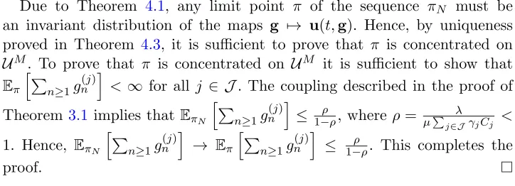
Table 2 Insensitivity of Scheme 1
λ Mean sojourn time ¯T
(Theoretical)
Constant
(Simulation)
Power Law
(Simulation)
0.2 0.8076 0.8106 0.8098
0.3 0.8609 0.8642 0.8640
0.5 0.9809 0.9852 0.9840
0.7 1.1696 1.1759 1.1757
0.8 1.3687 1.3741 1.3740
0.9 1.7531 1.7641 1.7645
1. Constant: We consider job length distribution having the cumulative distribution given byF(x) = 0 for 0≤x <1, andF(x) = 1, otherwise. 2. Power law: We consider job length distribution having cumulative dis-tribution function given byF(x) = 1−1/4x2 forx≥ 12 andF(x) = 0, otherwise.
For both distributions we have μ = 1. We choose the following parameter valuesM = 2,C1= 4/3,C2 = 2/3,N = 100,γ1 =γ2= 12, andd1=d2 = 2.
[image:25.612.180.425.356.487.2]7. Conclusion. We considered randomized job assignment schemes in a multi-server system consisting ofN parallel processor sharing servers, cate-gorized intoM (N) different types according to their processing capacity or speed. In the proposed schemes, a small number of servers from each type is sampled uniformly at random at each arrival instant. It was shown that due to such sampling the schemes achieve the maximal stability region. Mean field analysis was carried out to show that asymptotic independence among servers holds even when M is finite and exchangeability holds only within servers of the same type. The existence and uniqueness of stationary solution of the mean field and doubly exponentially decreasing nature of the tail distribution of the number of jobs was established. Numerical studies have shown that, when the estimates of arrival rates are not available, the proposed schemes offer simpler alternatives to achieving lower mean sojourn time of jobs.
APPENDIX A
We will prove Proposition4.1only for the system (4.1)–(4.2). The proof for the system (4.5)–(4.6) follows similarly.
Define θ(x) = [min(x,1)]+, where [z]+ = max{0, z} and let us consider
the following modification of (4.1)–(4.2):
u(0) =g,
(A.1)
˙
u(t) =ˆl(u(t)),
(A.2)
where the mappingˆl:RZ+M →RZ+M is given by
ˆ
l0(j)(u) = 0, forj∈ J,
(A.3)
ˆ
lk(j)(u) = λ
γj
θ
u(kj−)1
dj
−θ
u(kj)
dj
+
j−1
i=1
θ
u(ki−)1
di
(A.4)
× M
i=j+1
θ
u(ki)
di
−μCj
θ
u(kj)
−θ
u(kj+1)
+, fork≥1, j ∈ J.
Clearly, the right hand side of (4.4) and (A.4) are equal ifu∈U¯M. Therefore, the two systems must have identical solutions in ¯UM. Also ifg∈U¯M, then any solution of the modified system remains within ¯UM. This is because
of the facts that if u(nj)(t) = u(nj+1) (t) for some j, n, t, then ˆl (j)
n (u(t)) ≥ 0
and ˆl(nj+1) (u(t))≤0, and if u(nj)(t) = 0 for some j, n, t, then ˆln(j)(u(t)) ≥0.
that the modified system (A.1)–(A.2) has a unique solution in (RZ+)M. We
now extend the distance metric defined in (2.8) to the space (RZ+)M.
Using the metric defined in (2.8) and the facts that|x+−y+| ≤ |x−y|for
any x, y ∈R, |a1b1m−a2bm2 | ≤ |a1−a2|+m|b1−b2|for any a1, a2, b1, b2 ∈
[0,1], and|θ(x)−θ(y)| ≤ |x−y|for any x, y∈Rwe obtain
ˆl(u) ≤K1,
(A.5)
ˆl(u)−ˆl(w) ≤K2 u−w ,
(A.6)
whereu,w∈(RZ+)M,K
1 andK2 are constants defined asK1 = minjλ∈Jγj+
μ(maxj∈J Cj) andK2 = 4M λmaxminjj∈J∈Jγdjj+3μ(max1≤j≤MCj). The uniqueness
now follows from inequalities (A.5) and (A.6) by using Picard’s iteration technique since (RZ+)M is complete under the metric defined in (2.8).
APPENDIX B
We prove Proposition 4.2 by showing that the generators of the corre-sponding semigroups converge as N → ∞. We first recollect the following from [7].
• The generator AN of the semigroup {TN(t)}t≥0 acting on functions
f : Mj=1U¯N(j) → R is given by ANf(g) = h=gqgh(f(h)−f(g)), where qgh, with g,h ∈
M j=1U¯
(j)
N , denotes the transition rate from
stateg to stateh.
• The generator A of the semigroup {T(t)}t≥0 acting on functionsf : ¯
UM → R having bounded partial derivatives is given by Af(g) =
limt↓0 T(t)f(gt)−f(g) = dtdf(u(t,g))|t=0.
In the following lemma, we characterize the the generatorAN associated with the processxN(t).
Lemma B.1. Let g ∈ M j=1U¯
(j)
N be any state of the process xN(t) and e(n, j) =
e(ki)
k∈Z+,i∈J
be the unit vector withe(nj)= 1 andek(i)= 0 if i=j andk=n. Under Scheme 1, the generator AN of the Markov processxN(t) acting on functionsf :Mj=1U¯N(j)→R is given by
(B.1) ANf(g) =N λ M
j=1
n≥1
gn(j−)1
dj
−g(nj)
djj−1
i=1
gn(i−)1
di
× M
i=j+1
gn(i)
di
f(g+ e(n, j)
N γj
)−f(g)