ABSTRACT
MOMEN, MOSTAFA HASSAN. Complex Modulus Determination of Asphalt Concrete
Using Indirect Tension Test. (Under the direction of Dr. Y. Richard Kim).
The purpose of this research is to present the results from an analytical/experimental
study on the dynamic modulus testing of hot mix asphalt (HMA) using the indirect tension
(IDT) mode. The analytical solution for dynamic modulus determination in IDT was
developed by Kim (14) using the theory of linear viscoelasticity. To verify the analytical
solution, temperature and frequency sweep tests were conducted on 24 asphalt mixtures
commonly used in North Carolina, using both axial compression and IDT test methods. In
doing so, a modified dynamic modulus test protocol is introduced that reduces the required
testing time by using more frequencies and fewer temperatures based on the
time-temperature superposition principle. A comparison of results from the axial compression and
IDT test methods shows that the dynamic modulus mastercurves and shift factors derived
from the two methods are in good agreement. It was also found that Poisson’s ratio is a weak
function of the loading frequency; its effect on the phase angle mastercurve is discussed.
After verification of the analytical solution, another study was conducted to evaluate the
effect of aggregate size on the variability of test results, where the coefficient of variation
(CV) was computed for each aggregate size and the results were compared. It was found that
Complex Modulus Determination of Asphalt
Concrete Using Indirect Tension Test
BY
MOSTAFA MOMEN
A THESIS SUBMITTED TO THE GRADUATE FACULTY OF NORTH CAROLINA STATE UNIVERSITY
IN PARTIAL FULFILLMENT OF THE REQUIREMENTS FOR THE DEGREE OF
MASTER OF SCIENCE
DEPARTMENT OF CIVIL ENGINEERING
RALEIGH
2004
APPROVED BY:
DEDICATION
It is my honor to dedicate this thesis to my beloved wife for the support and love she
showed me throughout the two year journey of my graduate studies towards the Master of
Science degree. I would like also to dedicate this thesis to my father who encouraged me to
pursue a graduate degree and has been always there for me when I needed his guidance and
BIOGRAPHY
Mostafa Momen was born in Urbana-Champaign, ILLINOIS where he lived with his
parents for three years while his father was pursuing a Doctor of Philosophy degree in civil
engineering. In1982, he moved to United Arab Emirates with his family where he lived for
one year and attended kinder garden. In 1983, he moved to Egypt with his family and
attended Manor House School for 11 years from which he graduated in June 1994. In
September of 1994 the author enrolled in the American University in Cairo majoring in
construction engineering and management, and received a Bachelor of Science Degree in
June 1999. He traveled in August 1999 to United Arab Emirates where he worked for a
consulting company as a structural engineer for two years, and then he worked with his father
as an arbitration engineer for one and a half years. In December 2002 he decided to go back
to the United States to pursue a graduate degree in civil engineering. He enrolled in North
Carolina State University where he worked as a graduate research assistant under the
supervision of Dr. Y. Richard Kim. This led to the research contained herein and to this
ACKNOWLEDGEMENTS
First of all, I thank ALLAH for his guidance and support.
The author would like to thank the members of his advisory committee and all the
research group members for their help and guidance during his graduate studies. I also extend
a sincere appreciation for my advisor Dr. Y. Richard Kim for providing me the opportunity
to work with him as a research assistant and for his encouragement and technical assistance.
Special thanks to Mark King who helped me a great deal and he was also my partner and
dear friend throughout this whole process. I also would like to thank Dr. Ghassan Chehab,
Dr. Youngguk Seo, and Shane Underwood for their help to me in both my experimental and
analytical work.
Finally, my gratitude is extended to my parents, Hassan Momen and Faten Khalifa,
TABLE OF CONTENTS
LIST OF TABLES ...IX LIST OF FIGURES ... X LIST OF SYMBOLS AND ABBREVIATIONS ... XII
1. INTRODUCTION... 1
1.1 RESEARCH NEEDS... 1
1.2 RESEARCH OBJECTIVE AND SIGNIFICANCE... 2
1.3 THESIS ORGANIZATION... 3
2. THEORETICAL BACKGROUND ... 4
2.1 DYNAMIC MODULUS DETERMINATION IN IDT ... 4
2.1.1 Linear Elastic Solution ... 4
2.1.2 Linear Viscoelastic Solution ... 5
2.2 CREEP COMPLIANCE CALCULATION IN IDT... 11
2.3 DETERMINATION OF CENTER POINT STRAIN FROM HORIZONTAL DEFORMATION.... 14
3. SPECIMEN PREPARATION AND EXPERIMENTAL PROGRAM... 16
3.1 SPECIMEN PREPARATION... 16
3.1.1 Asphalt Concrete Mixtures ... 16
3.1.2 Target Air Voids... 18
3.1.3 Maximum Specific Gravity Determination ... 18
3.2 EXPERIMENTAL PROGRAM... 19
3.2.1 Testing System... 19
3.2.2 Test Protocol... 21
4. DATA ANALYSIS AND RESULTS ... 25
4.1 DATA ANALYSIS... 25
4.1.1 Software ... 25
4.1.2 Mastercurve Construction ... 26
4.1.2.1 Dynamic Modulus... 26
4.1.2.2 Phase Angle and Poisson’s Ratio... 27
4.2 RESULTS... 28
4.2.1 Dynamic Modulus ... 28
4.2.2 Shift Factor ... 29
4.2.3 Phase Angle and Poisson’s Ratio ... 31
5. COMPARISON BETWEEN IDT AND AXIAL COMPRESSION TEST RESULTS 35 5.1 DYNAMIC MODULUS... 35
5.1.1 Graphical Comparison ... 35
5.1.2 Statistical Analysis... 40
5.1.2.1 Using P-Value... 40
6.1 DIGITAL IMAGE CORRELATION (DIC)... 45
6.1.1 Test Method... 46
6.1.1.1 Test Protocol ... 46
6.1.1.2 Testing Equipment ... 47
6.1.1.3 Test Setup... 47
6.1.2 Data Analysis ... 48
6.1.2.1 Data Acquisition and Analysis Software ... 48
6.1.2.2 Area of Interest ... 48
6.1.2.3 Seed Point ... 50
6.1.2.4 Strain Calculation... 50
6.1.3 Test Results ... 51
6.1.3.1 S 9.5C-Fine Mix... 51
6.1.3.1.1 Vertical Strains... 52
6.1.3.1.2 Horizontal Strains ... 53
6.1.3.2 B 25.0C-Fine Mix ... 56
6.1.3.2.1 Vertical Strains... 57
6.1.3.2.2 Horizontal Strains ... 59
6.2 STATISTICAL ANALYSIS... 63
6.2.1 Standard deviation... 63
6.2.2 Coefficient of Variation... 63
7. CONCLUSIONS ... 65
REFERENCES... 67
A.1DYNAMIC MODULUS... 71
A.2PHASE ANGLE... 83
APPENDIX B: PHOTOGRAPHS... 89
B.1TESTING SYSTEM... 90
B.2TEST SETUP... 91
B.3TESTING JIG... 92
APPENDIX C: IDT DYNAMIC MODULUS DATA BASE... 93
C.1DYNAMIC MODULUS CALCULATION... 94
LIST OF TABLES
Table 2.1 Coefficients for Poisson’s Ratio and Dynamic Modulus... 10
Table 2.2 Coefficients Used to Calculate Poisson’s Ratio and Creep Compliance... 13
Table 2.3 Coefficients in Eq. (2-42) ... 15
Table 3.1 Information on Asphalt Mixtures Tested in This Study ... 17
Table 3.2 Comparison of the NCHRP 1-37A and Modified Test Protocols ... 22
LIST OF FIGURES
Figure 2.1 Schematic of the IDT Specimen Subjected to a Strip Load ... 6
Figure 3.1 (a) IDT Test Setup with SHRP LGD; (b) Surface-Mounted LVDTs... 20
Figure 3.2 Comparison of Mastercurves Between Three-Temperature (empty symbols) and Five-Temperature (filled symbols) Testing for S9.5C–Fine Mixture ... 23
Figure 4.1 Frequency Dependent Electronic Phase Angle for MTS ... 28
Figure 4.2 S 9.5C Fine Mixture Replicates Mastercurves ... 29
Figure 4.3 S 9.5C Fine Mixture Dynamic Modulus Mastercurve ... 30
Figure 4.4 Shift Factor as a Function of Temperature ... 30
Figure 4.5 Vertical and Horizontal Phase Angles Mastercurve... 32
Figure 4.6 Poisson’s Ratio Mastercurve ... 32
Figure 4.7 Poisson’s Ratio for 9.5 mm Mixtures... 33
Figure 4.8 Poisson’s Ratio for 12.5 mm Mixtures... 33
Figure 4.9 Poisson’s Ratio for 19.0 mm Mixtures... 34
Figure 4.10 Poisson’s Ratio for 25.0 mm Mixtures... 34
Figure 5.1 Dynamic modulus master curves for: (a) S9.5A-Fine mixture; (b) S9.5B-Coarse mixture; (c) S9.5C-Fine mixture; (d) S9.5C-Coarse mixture... 37
Figure 5.2 Dynamic modulus master curves for: (a) S12.5C-Fine mixture; (b) S12.5D-Coarse mixture; (c) I19.0B-Fine mixture; (d) I19.0C-Coarse mixture... 38
Figure 5.3 Dynamic modulus master curves for: (a) I19.0D-Fine mixture; (b) I19.0D-Coarse mixture; (c) B25.0B-Fine mixture; (d) B25.0B-Coarse mixture... 39
Figure 5.4 S9.5A-Fine Mixture Phase angle mastercurves... 43
Figure 5.5 I19.0D-Fine mixture Phase Angle Mastercurves ... 44
Figure 6.1 Vertical Area of Interest ... 49
Figure 6.2 Horizontal Area of Interest... 49
Figure 6.8 Point Strain Profile along Vertical Axis... 55
Figure 6.9 Point Strain Profile along Horizontal Axis... 56
Figure 6.10 Aggregate Orientation on the Surface of the Specimen ... 57
Figure 6.11 Vertical Strain Field Measurement along the Vertical Axis ... 58
Figure 6.12 Vertical Strain Field Measurement along the Horizontal Axis ... 58
Figure 6.13 Horizontal Strain Field Measurement along the Vertical Axis ... 60
Figure 6.14 Horizontal Strain Field Measurement along the Horizontal Axis ... 61
Figure 6.15 Point Strain Profile along Vertical Axis... 62
Figure 6.16 Point Strain Profile along Horizontal Axis... 62
LIST OF SYMBOLS AND ABBREVIATIONS
• σ: Stress
• ε: Strain
• υ: Poisson’s Ratio
• E* : Dynamic Modulus
• φ: Phase Angle
• PG: Performance Grade
• NMSA: Nominal Maximum Size Aggregate
• LVDT: Linear Variable Differential Transformer
• LGD: Load Guide Device
• SHRP: Strategic Highway Research Program
• fR: Reduced Frequency
• DIC: Digital Image Correlation
1. INTRODUCTION
1.1 Research Needs
The design methods adopted in the NCHRP 1-37A Design Guide (3) are based on
mechanistic-empirical principles in which the prediction of pavement responses and
performance must take into account fundamental properties of layer materials. Among these,
the most important property, but a relatively new concept to state highway agencies, is the
dynamic modulus of asphalt concrete. This property represents the temperature and
frequency (and, therefore, time) dependent stiffness characteristics of the material.
Recently, a significant amount of effort has been given to the development of a test
protocol to determine the dynamic modulus of HMA. This effort has resulted in a standard
test protocol that can be used for the NCHRP 1-37A Design Guide (3). This test protocol
calls for the use of axial compression testing for measuring the dynamic modulus.
One of the issues related to the dynamic modulus is its use in forensic studies and
pavement rehabilitation design. The current dynamic modulus protocol calls for the axial
compression testing of 100 mm diameter and 150 mm tall asphalt concrete specimens. It is
often impossible to obtain this size specimen from actual pavements. Given that a typical
asphalt layer thickness is less than a few inches and that coring is the most effective method
of obtaining specimens from actual pavements, the Indirect Tension (IDT) testing of cores
differences between the axial compression and IDT tests raise questions about the
interchangeability of the dynamic modulus values obtained from the two test methods.
Two major differences between these two test methods are:
1. State of stress: Compression testing creates the uniaxial state of stress, whereas the
stress state in the IDT test is biaxial; and
2. The relationship between compaction direction and the direction in which the
stress-strain analysis is performed: In axial compression these two directions are the same,
whereas in IDT these two directions are perpendicular. The anisotropy that may exist
in the Superpave Gyratory Compactor specimen amplifies the effect of this
difference.
1.2 Research Objective and Significance
Recognizing the importance of the IDT dynamic modulus test for the pavement
industry, these issues were investigated by an analytical/experimental study at North Carolina
State University. The objective of this research is to document the findings from this study,
which may serve as an important foundation for developing a standard test protocol for the
IDT dynamic modulus test. The research presented herein was conducted as part of the
NCDOT research project HWY 2003-09 entitled “Typical Dynamic Modulus Values of
Asphalt Concrete Mixtures.”
indirect tension testing on Superpave Gyratory compacted specimens simulates the
relationship between the compaction direction and critical tensile stress direction in the field
accurately. These advantages support the significance of using indirect tension specimens to
determine the dynamic modulus of asphalt concrete mixtures.
1.3 Thesis Organization
This thesus is composed of seven chapters. Chapter 1 presents the research needs and
the objectives to be achieved. Theoretical background and literature review about the indirect
tension test is presented in Chapter 2. Chapter 3 includes the description of the materials used
in the study, the specimen preparation methods, and the experimental program. Chapter 4
presents the laboratory testing results and analysis. Verification of test results is presented in
Chapter 5 by comparing IDT dynamic modulus and phase angle test results to those
determined from the axial compression mode and evaluating how different the results are
using statistical analysis. Chapter 6 presents the effect of aggregate size on the variability of
test results. Finally, Chapter 7 presents the conclusions of this research and suggestions for
2. THEORETICAL BACKGROUND
2.1 Dynamic Modulus Determination in IDT
2.1.1 Linear Elastic Solution
Since Hondros (4) derived elastic solutions for the IDT test using the plane stress
assumption, the pavement community used those solutions until Roque and Buttlar (11, 12)
introduced correction factors that take into account the bulging effect of the specimen. Then,
Kim and Wen (15) introduced viscoelastic solutions for the IDT creep test using the theory of
linear viscoelasticity.
Unlike the uniaxial test, the stress and strain distributions in the IDT specimen are
biaxial in nature. This biaxial state of stress and strain can cause errors in determining the
material properties from the IDT test unless the derivation of the properties is carefully
handled. These errors may cause enough difference between the dynamic modulus
determined from the IDT test and that from the axial compression test that the criteria and
design methods based on the dynamic modulus determined from the axial compression test
cannot be used in forensic studies where the asphalt layer is not thick enough to yield 150
mm tall specimens to be used in axial compression testing.
Uniaxial case: σy =E×εy or
E
y y
σ
ε = (2-1)
Biaxial case: x 1 ( x y)
E σ νσ
ε = − (2-2)
where x and y denote the loading direction (i.e., the vertical direction) and the direction
perpendicular to the loading direction (i.e., the horizontal direction), respectively.
In the uniaxial case (i.e., the axial compression dynamic modulus test) in Eq. (2-1),
one can divide the axial stress (σy) by the axial strain (εy) to obtain the modulus. However, in
the biaxial case (i.e., the IDT dynamic modulus test) in Eq. (2-2), one cannot obtain the
modulus by dividing the horizontal stress (σx) by the horizontal strain (εx). Rather, the correct
way to determine the modulus of the material is to divide the biaxial stress (i.e., σx-νσy) by
the horizontal strain (εx). If the incorrect solution (i.e., σx/εx) is used to represent the modulus
of the material, it should not be considered the same as the modulus determined from the
axial test.
2.1.2 Linear Viscoelastic Solution
The linear viscoelastic solution for the complex modulus of HMA under the IDT
mode has been developed by Kim et al. (14) and is presented in this section. This solution
will be applied to the IDT test results to evaluate its accuracy against the dynamic modulus
determined by the axial compression test. A comparison between both elastic and
viscoelastic solutions in IDT will be presented.
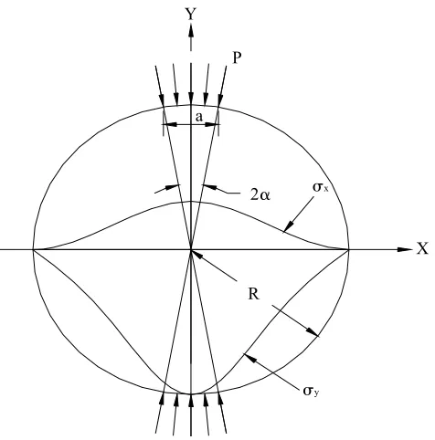
Assuming the plane stress state, Hondros (4) developed the following expressions for
stresses and strains along the horizontal diameter of the IDT specimen subjected to a strip
Y σy a R 2α P σx X
Figure 2.1 Schematic of the IDT specimen subjected to a strip load ) ( 1 y x x
E σ νσ
ε = − (2-3)
with
[
( ) ( )]
2 tan / 1 / 1 tan / 2 cos / 2 1 2 sin ) / 1 ( 2 )( 2 2
2 2 1 4 4 2 2 2 2 x g x f ad P R x R x R x R x R x ad P x
x = −
+ − − + + − = − π α α α π
σ (2-4)
[
( ) ( )]
2 tan / 1 / 1 tan / 2 cos / 2 1 2 sin ) / 1 ( 2 )( 2 2
2 2 1 4 4 2 2 2 2 x g x f ad P R x R x R x R x R x ad P x
y =− +
+ − + + + − − = − π α α α π
σ (2-5)
where
P = applied load
a = loading strip width, m
ν = Poisson’s ratio
For the viscoelastic materials subjected to the sinusoidal load in a steady state, Eq.
(2-3) can be rewritten as:
) (
1
* x y
x
E σ νσ
ε = − (2-6)
where E*is the complex modulus. It is often helpful to have E* in polar form,
φ i
e E
E* = * ⋅ (2-7)
where E* is the dynamic modulus and φ is the phase angle calculated from the time lag
between the load and the displacement. The response to the sinusoidal load applied in the
complex modulus test is the imaginary component of the response due to the complex load,
P, shown below:
) sin (cos
0
0e P wt i wt
P
P= iwt = + (2-8)
where P0 and w are the amplitude and the angular frequency of the sinusoidal load used in
the complex modulus test, respectively.
Substituting Eqs. (2-4), (2-5), (2-7), and (2-8) into Eq. (2-6) results in:
[
(1 ) ( ) ( 1) ( )]
2) ,
( ( )
*
0 e f x g x
ad E
P t
x iwt
x = + + −
− ν ν
π
ε φ (2-9)
Integrate Eq. (2-9) over the gauge length to determine the horizontal displacement, U(t), and
obtain: − + + = =
∫
∫
∫
− − − − l l l l wt i l lx e f x dx g x dx
ad E P dx t x t
U( ) ( , ) 2 ( ) (1 ) ( ) ( 1) ( )
*
0 ν ν
π
where l is half of the gauge length. One may extract the response that only occurs due to the
sinusoidal input by taking an imaginary part of the total response. Therefore, the dynamic
modulus from the horizontal displacement, U(t), can be expressed as:
A t U ad wt P E ) ( ) sin( 2 0 * ⋅ − = π φ (2-11) where − + + =
∫
∫
− − l l l l dx x g dx x fA (1 ν) ( ) (ν 1) ( ) (2-12)
with
( )
(
2 22 2)
4 42 2 1 2 1 R / x cos R / x sin R / x x f + + − = α
α and (2-13)
( )
+ −= − tanα
R / x R / x tan x
g 2 2
2 2 1
1
1 (2-14)
Similarly, the analogous expression for the dynamic modulus from the vertical
displacement, V(t), can be derived as:
B t V ad wt P E ) ( ) sin( 2 0 * ⋅ − = π φ (2-15) where + − − =
∫
∫
− − l l l l dy y m dy y nB (ν 1) ( ) (1 ν) ( ) (2-16)
with
By equating Eqs. (2-11) and (2-15), one can obtain
) ( )
(t B U t V
A⋅ = ⋅ (2-19)
Then, one may derive the expression for Poisson’s ratio as follows:
) ( ) ( ) ( ) ( 2 2 1 1 t V t U t V t U γ β γ β ν + − − = (2-20) where
∫
∫
− − − − = l l l l dy y m dy yn( ) ( )
1 β ,
∫
∫
− − − = l l l l dy y m dy yn( ) ( )
2 β ,
∫
∫
− − − = l l l l dx x g dx xf( ) ( )
1
γ , and
∫
∫
− − + = l l l l dx x g dx xf( ) ( )
2
γ (2-21)
Combining Eqs. (2-11) and (2-15) yield a single form of the dynamic modulus, as
shown below: ) ( ) ( ) ( ) sin( ) ( ) sin( 0 0 * t U t V ad t BU wt P t AV wt P E ⋅ ⋅ − + − = π φ φ (2-22)
After substituting Eqs. (2-12) and (2-16) into Eq. (2-22), one can obtain:
) ( ) ( ) sin( 2 2 2 1 2 2 1 0 * t U t V ad wt P E β γ γ β γ β π φ − − −
= (2-23)
The vertical and horizontal displacements can be expressed in sine functions as follows:
) sin(
)
(t =V0 wt−φ
) sin(
)
(t =U0 wt−φ
U (2-24b)
where V0 and U0 are the constant amplitudes of vertical and horizontal displacements,
respectively. Therefore, the final form of the dynamic modulus is:
0 2 0 2 1 2 2 1 0 * 2 U V ad P E β γ γ β γ β π − − = (2-25)
Likewise, the expression for Poisson’s ratio can be simplified as:
0 2 0 2 0 1 0 1 V U V U γ β γ β ν + − −
= (2-26)
The coefficients, β1, β2, γ1, and γ2, in Eqs. (2-25) and (2-26), are calculated for
different specimen diameters and gauge lengths, and are presented in Table 2.1. Eqs. (2-25)
and (2-26) are based on the plane stress assumption. Kim and Wen (15) used the
three-dimensional finite element analysis to calculate the center strain in the IDT specimen and
concluded that the error due to the plane stress assumption is negligible.
Table 2.1 Coefficients for Poisson’s Ratio and Dynamic Modulus
Specimen
Diameter (mm) Gauge Length (mm) β1 β2 γ1 γ2
101.6 25.4 -0.0098 -0.0031 0.0029 0.0091
101.6 38.1 -0.0153 -0.0047 0.0040 0.0128
101.6 50.8 -0.0215 -0.0062 0.0047 0.0157
152.4 25.4 -0.0065 -0.0021 0.0020 0.0062
152.4 38.1 -0.0099 -0.0032 0.0029 0.0091
2.2 Creep Compliance Calculation in IDT
Following Hondros’s analysis, Eqs. (2-3), (2-4), and (2-5) can be used to express
stresses and strains along the horizontal diameter of the specimen. Due to the viscoelastic
characteristics of asphalt concrete, strain is also time dependent. The elastic-viscoelastic
correspondance was used to solve the viscoelastic problem. The principle states that the
viscoelastic equations are similar to the elastic equations in the Laplace transformed domain
with the substitution of the Carson transformed modulus for the elastic modulus. Poisson’s
ratio is assumed to be constant. Thus, the transformed form of the stress-strain relationship is:
( )
ε_ ~ σ σ _ _ , x s E v x y= 1 − (2-27)
where
ε
_ ,σ
_x, andσ
_yare Laplace transformed strain and stresses whileE
~ is the Carsontransformed modulus. According to the theory of viscoelasticity, the relationship between the
relaxation modulus and creep compliance is:
E D~ × ~ =1 (2-28)
where
D
~ is the Carson transformed creep compliance. SubstituteE
~ withD
~ , and Eq. (5-4)becomes: ) ( ) , ( ~ _ _ _ y x v D s
x σ σ
ε = − (2-29)
Eqs. (2-4), (2-5), and (2-29) yield:
[
(1 ) ( ) ( 1) ( )]
2 ) , ( ( ) _ ~ _ x g x f e ad P D sx = i wt− +ν + ν −
π
where P = PoH(t) for a creep test and
H(t) = 0, when t<0; 1, when t>0
Taking the inverse Laplace transform on both sides of Eq. (2-30) yields:
[
]
τ τ τ ν ν π ε d d dP t D x g x f ad t x t x = + + −∫
−0 ) ( ) ( ) 1 ( ) ( ) 1 ( 1 ) , ( (2-31)
Eq. (2-31) becomes:
[
(1 ) ( ) ( 1) ( )]
) ( 2 ) ,
( 0 D t f x g x
ad P t x
x =π +ν + ν −
ε (2-32)
The horizontal deformation U(t) is obtained by integrating the strain over the entire gauge
length:
∫
− = l l dx t x tU( ) ε( , ) (2-33)
where l is half of the gauge length. Eqs. (2-32) and (2-33) yield:
− + + =
∫
∫
− − l l l l dx x g dx x f ad E t D P tU( ) 2 ( ) (1 ) ( ) ( 1) ( )
*
0 ν ν
π (2-34)
Rearranging Eq. (2-34) for creep compliance, D(t), yields:
A P t U t D o 2 ) ( )
( = (2-35)
Similarly, the analogous expression for the creep compliance from the vertical
displacement, V(t), can be derived as:
B P t V t D o 2 ) ( )
( = (2-37)
where + − − =
∫
∫
− − l l l l dy y m dy y n adB 1 (ν 1) ( ) (1 ν) ( )
π (2-38)
Eqs. (2-35) and (2-37) yields:
) ( ) ( ) ( ) ( 2 2 1 1 t V b t U a t V b t U a + + − =
ν (2-39)
[
( ) ( )]
)( cU t eV t
p d t
D =− + (2-40)
where a1, a2, b1, b2, c, and e are coefficients related to specimen diameter and gauge length
used to measure displacements. Note that Eq. (2-39) has the same form as Eq. (2-20). Values
of these coefficients for various specimen diameter and gauge length are presented in Table
2.2. One may observe that the coefficients in Table 2.1 and Table 2.2 are different but they
will yield the same Poisson’s ratio for any given specimen geometry.
Table 2.2 Coefficients Used to Calculate Poisson’s Ratio and Creep Compliance
25.4 3.385 1.081 1 3.122 0.7874 2.2783
50.8 4.58 1.316 1 3.341 0.4032 1.024
25.4 3.172 1.039 1 3.06 1.199 35.33
50.8 3.673 1.154 1 3.192 0.611 1.685
76.2 4.559 1.33 1 3.311 0.475 1.034
c e
a1 a2 b1 b2
It is note worthy that Eq. (2-40) is independent of Poisson’s ratio and, thus, is
material independent. This is due to the two-dimensional plane stress assumption used in the
derivation. Poisson’s ratio cannot be deleted from Eq. (2-40) if the viscoelastic solution was
based on a three-dimensional solution.
2.3 Determination of Center Point Strain from Horizontal Deformation
Knowing that the maximum tensile strain along the horizontal axis occurs at the
center point of the specimen and that the failure plane is along the vertical axis, the measured
deformation across a given gauge length must be converted into a center point strain, instead
of the average strain that is measured using the LVDT’s, in order to study the stress-strain
relationship of the element where the crack is initiated.
Using Eq. (2-32) and the theory of viscoelasticity, along the horizontal diameter of
the IDT specimen, the center point strain, εx=0, in a creep test is represented as follows:
[
(1 ) ( 0) ( 1) ( 0)]
) ( 2 )
( 0
0 = + = + − =
= D t f x g x
ad P t
x π ν ν
ε (2-41)
Eqs. (2-34) and (2-41) yield:
UA dv c
bv a U
x + =
+ = =0
ε (2-42)
where a, b, c, and d are coefficients related to specimen diameter and gauge length used.
Table 2.3 Coefficients in Eq. (2-42)
One can observe from Eq. (2-42) that the strain-deformation relationship is
independent of stress and dependent on Poisson’s ratio. Thus, Eq. (2-42) can be applied to
specimens subjected to any loading conditions. The dependency on Poisson’s ratio is due to
the plane stress assumption along the thickness of the specimen, however, the dependency is
insensitive to the change in Poisson’s ratio.
25.4 12.4 37.7 0.291 0.908
50.8 12.4 37.7 0.471 1.57
25.4 8.48 25.6 0.207 0.634
50.8 8.48 25.6 0.373 1.18
76.2 8.48 25.6 0.478 1.59
100
150 Specimen Diameter (mm)
Gauge
3. SPECIMEN PREPARATION AND EXPERIMENTAL PROGRAM
3.1 Specimen Preparation
3.1.1 Asphalt Concrete Mixtures
Twenty four different North Carolina mixtures were used in this project to verify the
viscoelastic solutions for the dynamic modulus in IDT. All the aggregates used were granite
from six different sources in North Carolina. Four different nominal maximum aggregate
sizes were used: 9.5, 12.5, 19, and 25 mm. Three different PG grades were used (PG 64-22,
PG 70-22, and PG 76-22) from six different sources. Table 3.1 shows the details of the
asphalt concrete mixtures used.
The mixing and compaction temperatures for PG 64-22, PG 70-22, and PG 76-22
Table 3.1 Information on Asphalt Mixtures Tested in This Study
Note: aS for surface mix, I for intermediate mix, and B for base mix
bIndicates the nominal maximum size of aggregate in mm (Superpave mix
designation)
cTraffic volume indicator (A: lowest traffic, D: highest traffic)
dAggregate gradation (F: Fine, C: Coarse, 1: Fine)
# Binder Mixture
Asphalt
content % Binder Source Aggregate Quarry
Aggregate
3.1.2 Target Air Voids
The target air voids for all specimens tested in this project was 4%. A small study was
conducted using four mixtures with different NMSA to estimate the reduction in air voids
when the specimen is cut from 60 mm height to 38 mm. The study showed that in general the
reduction in air voids would be around 1% for 9.5 mm NMSA and it would increase by
approximately 0.5% increment as the NMSA increases to 12.5, 19, and 25 mm.
3.1.3 Maximum Specific Gravity Determination
The maximum specific gravity (Gmm) of all mixtures was measured according to
AASHTO TP34-94, commonly known as Rice Specific Gravity. Appropriate correction
factors were applied to correct for the specific gravity of water when the temperature of
water is different than 25°C. Three replicates were used to determine the Gmm of each
mixture by averaging the values obtained from the replicates. Maximum error allowed
between replicates was 0.011 according to the specification.
3.1.4 Specimen Fabrication
Three gyratory specimens for each mixture were prepared to 60 mm height and 150
mm diameter, and they were cut to 38 mm height. In order to achieve the target air void
3.2 Experimental Program
3.2.1 Testing System
Testing was performed using a closed-loop servo-hydraulic machine, manufactured
by MTS, using a 5 kip load cell, that is capable of applying load over a wide range of
frequencies ranging from 0.01 Hz to 25 Hz. The temperature control system of MTS is based
on the use of low pressure liquid nitrogen to condition the chamber where the specimen is
being tested. The temperature control system is able to achieve the required testing
temperatures ranging from -10°C to 35°C. An asphalt concrete dummy specimen with similar
geometry and a temperature probe (thermocouple) embedded in the middle of the specimen
was placed inside the chamber in order to monitor the actual temperature of the specimen
during testing.
The data acquisition system for MTS is fully computerized and is capable of
measuring and recording data from several channels simultaneously. Six channels were used
in IDT dynamic modulus testing: two for vertical displacements, two for horizontal
displacements, and one for load cell, one for actuator. Data acquisition programs were
prepared using Labview software for data collection and analysis.
The vertical and horizontal deformations were measured using linear variable
differential transformers (LVDTs). For IDT testing, two loose core type miniature XSB
LVDTs were mounted on each of the specimen faces using a 50.8 mm gauge length (2 inch),
as shown in Figure 3.1(b)
The Load Guide Device (LGD), developed from the Strategic Highway Research
Figure 3.1(a). From the NCHRP 1-28 study, it was found that when compared against other
loading devices with no column or four columns, the SHRP LGD with two guide columns
resulted in the least amount of “rocking” of the IDT specimen without causing significant
friction between the upper loading plate and guide columns under repetitive loading (16).
Figure 3.1 (a) IDT test setup with SHRP LGD; (b) Surface-Mounted LVDTs
3.2.2 Test Protocol
The NCHRP 1-37A draft protocol provides recommended testing temperatures and
frequencies, summarized in Table 3.2. It was recognized that this test protocol could be
simplified by reducing the number of testing temperatures and increasing the number of
testing frequencies without compromising the mastercurve construction. The result of this
action could mean that the required testing time to obtain a mastercurve would decrease
because of the reduced amount of temperature conditioning. This reduced testing time could
provide a significant benefit to practicing agencies. The test protocol proposed by the
NCHRP 1-37A project takes 11 to 12 hours to complete using the liquid nitrogen temperature
chamber. This amount of time is more than one working day. The major portion of this
period is consumed by temperature conditioning time. It would take longer than 12 hours if a
refrigeration type chamber is used. The modified test protocol, however, takes less than 8
hours and, therefore, allows the completion of one dynamic modulus test within one working
day.
The underlying principle that allows the modification of the original test protocol is
the concept of time-temperature superposition (or time-temperature equivalence); that is, the
same modulus value of a material can be obtained either at low test temperatures and long
times or at high test temperatures but short times. The material that exhibits this type of
behavior is called thermorheologically simple (TRS).
Since the mastercurve development combines the effect of testing frequency and
temperature into one variable, called reduced frequency, it is possible to modify the range of
frequency in each temperature to compensate for the modification in the number of test
and the decrease in the number of testing temperatures, as shown in Table 3.2 under the
modified test protocol. A small study was conducted to verify the similarity of test results
between the two test protocols by testing in uniaxial mode.
Table 3.2 Comparison of the NCHRP 1-37A and Modified Test Protocols
Test Protocol No. of Temps. Test Temperatures (°C) Testing Frequencies (Hz) NCHRP 9-19 5 54.4, 37.8, 21.1, 4.4, -10 25, 10, 5, 1, 0.5, 0.1
NCSU 3 35, 10, -10 25, 10, 5, 1, 0.5, 0.1, 0.05, 0.01
One key requirement in developing a dynamic modulus mastercurve is to have an
overlap of the dynamic modulus vs. frequency curves between adjacent testing temperatures.
Figure 3.2 illustrates mastercurve development based on the 1-37A protocol of five testing
temperatures and the modified protocol of three temperatures. To develop this curve, the
dynamic modulus vs. frequency plot at various temperatures is horizontally shifted along the
frequency axis in a logarithmic scale to form a single curve at a reference temperature. The
first step involved in the determination of shift factors is to determine the frequencies at the
reference temperature and the temperature in question that yield the same dynamic modulus
values. Since the horizontal shift is performed on the logarithmic scale, the shift factor is then
determined by calculating the ratio of the frequency at the reference temperature to the
frequency at the temperature in question. After the horizontal shift, the frequency at the
reference temperature is then called reduced frequency. Therefore, to find the frequencies at
two temperatures that yield the same dynamic modulus values, it is necessary for the data to
0 10000 20000 30000 40000
0.000001 0.0001 0.01 1 100 10000 1000000
Reduced Frequency, Hz
IE
*I, M
P
a
-10C 4.4C 21.1C 37.8C 54.4C -10C 10C 35C
Figure 3.2 Comparison of mastercurves between three-temperature (empty symbols) and five-temperature (filled symbols) testing for S9.5C–Fine Mixture
The filled symbols in Figure 3.2 illustrate the overlap while using the 1-37A protocol.
It is noted that extra duplication of data exists at the lowest modulus or highest temperature
values. The empty symbols in Figure 3.2 show the overlap between adjacent temperatures
while using the three-temperature protocol. It can be seen from Figure 3.2 that, by adding
two low frequencies (0.05 and 0.01 Hz), sufficient overlap exists between temperatures. The
overlap is similar to that seen in five-temperature testing (filled symbols) between -10°C and
4.4°C or 4.4°C and 21.1°C. Some of the extra replication at the higher temperatures does not
exist in the three-temperature test data, which does not affect the quality of the overlap
Another important factor to consider in this comparison is the similarity between
dynamic modulus mastercurves from the two protocols. Each point in Figure 3.2 represents
the average of three replicates. When the average curves are compared, there is little
discrepancy between the protocols. This observation was verified for two different mixtures.
This finding suggests that one can use the three-temperature test protocol, which requires a
shorter testing time, and obtain the same dynamic modulus data as the five-temperature test
protocol would yield. All the IDT dynamic modulus tests in this project were conducted
according to the three-temperature test protocol.
The number of test replicates was three for each mixture type. In each frequency and
temperature combination of the three-temperature protocol shown in Table 3.2, the applied
load level was adjusted so that the resulting horizontal strain in the IDT specimen is between
4. DATA ANALYSIS AND RESULTS
4.1 Data Analysis
4.1.1 Software
LVDT and load cell measurements were collected using a National Instruments data
acquisition board and LabView software. The raw data were previewed before any analysis
was begun to ensure that the horizontal strain readings were within the target range (between
50 and 80 microstrains) and that all of the LVDTs read properly. Averaged deformations
were used to calculate the dynamic modulus and phase angle. In IDT, the vertical
deformations and horizontal deformations from two surfaces were averaged to determine the
deformation along each axis.
LabView software was used in determining the amplitudes of the sinusoidal load and
deformation histories. This program uses the Levenberg-Marquardt algorithm which is a
least squares approach to curve fitting. The last five cycles of data were analyzed and fitted
according to the following functional form:
) cos( )
(t =a+bt+c ωt+φ
f (4-1)
where f(t) is load or deformation time history;
a, b, and c are regression coefficients; φ is the phase angle; and
Coefficient c represents the amplitude of the sinusoidal waveform, and the dynamic modulus
is then calculated from the ratio of these coefficients from load and deformation histories.
The difference in the phase angles from the load and deformation analyses represents the
phase angle of the material.
The Labview software was programmed at North Carolina State University to utilize
the viscoelastic solution derivation in IDT to calculate the dynamic modulus and Poisson’s
ratio.
4.1.2 Mastercurve Construction
4.1.2.1 Dynamic Modulus
To construct a mastercurve the dynamic modulus vs. frequency curves at various
temperatures are horizontally shifted along the frequency axis in a logarithmic scale to form a
single curve at a reference temperature which was 10oC. The first step involved in the
determination of shift factors is to determine the frequencies at the reference temperature and
the temperature in question that yield the same dynamic modulus values. Since the horizontal
shift is performed on the logarithmic scale, the shift factor is then determined by calculating
the ratio of the frequency at the reference temperature to the frequency at the temperature in
question. After the horizontal shift, the frequency at the reference temperature is called
) (log
exp 1 1
*
R
f e d
b a
E Log
+ + +
= (4-2)
The mastercurve was constructed using the averaged dynamic modulus values from the three
replicates tested in each mixture. A detailed procedure is outlined in Appendix C to calculate
dynamic modulus for any of the mixtures tested in this study using the sigmoidal function
and the shift factor equation.
4.1.2.2 Phase Angle and Poisson’s Ratio
Phase angle is the time delay between stress and strain, and it is measured in degrees.
In order to determine the phase angle in IDT tests, the electronic and mechanical phase lags
due to machine compliance and electronic noise from the LVDT’s had to be determined first.
An aluminum specimen with same dimensions as IDT specimens was tested using the same
testing protocol used for dynamic modulus testing. Since aluminum is an elastic material, it
should exhibit no phase angle. The electronic phase angle values obtained from this test were
subtracted from those obtained from testing asphalt concrete specimens. It was found that
electronic phase angles were a function of frequency only and that temperature had a
negligible effect. Electronic phase angle values are presented in Figure 4.1. Then, the phase
angle mastercurves were developed using the shift factors determined from the construction
of the dynamic modulus mastercurves. In IDT two phase angle mastercurves were plotted,
the first is the “vertical phase” which is the phase angle between stress and vertical strain, the
second is the “horizontal phase” which is the phase angle between stress and horizontal
strain. It was discovered that the horizontal phase angles were always higher than the vertical
developed using the shift factors determined from the construction of the dynamic modulus
mastercurves.
0 5 10 15 20 25
0.001 0.01 0.1 1 10 100
Frequency
P
has
e A
ngl
e
Horizontal phase Vertical phase
Figure 4.1 Frequency dependent electronic phase angle for MTS
4.2 Results
In this section results from S 9.5C-Fine mixture is presented for demonstration
purposes, while the results for the remaining 23 mixtures could be found in Appendix A in a
graphical format. Also plotted in these figures are the axial compression data.
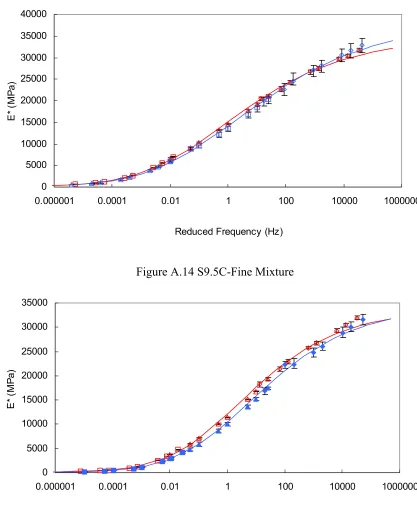
values from each replicate were averaged and a single mastercurve representing the mixture
was plotted in Figure 4.3.
4.2.2 Shift Factor
The reference temperature that was used as the basis for shifting the data was 10oC. A
quadratic equation was used to fit the three shift factor values obtained. Figure 4.4 shows a
shift factor plot against temperature.
0 5000 10000 15000 20000 25000 30000 35000
0.000001 0.0001 0.01 1 100 10000 1000000
Reduced Frequency (Hz)
E*
(
M
P
a)
-10C Rep. 1 10C Rep. 1 35C Rep. 1 -10C Rep. 2 10C Rep. 2 35C Rep. 2 -10C Rep. 3 10C Rep. 3 35C Rep. 3
0 5000 10000 15000 20000 25000 30000 35000
0.000001 0.0001 0.01 1 100 10000 1000000
Reduced Frequency (Hz)
E*
(
M
P
a)
-10 C Averaged 10 C Averaged 35 C Averaged Fit
Figure 4.3 S 9.5C-Fine mixture dynamic modulus mastercurve
y = 0.00056x2 - 0.15630x + 1.52179
R2 = 1.00000
-4 -3 -2 -1 0 1 2 3 4
-15 -5 5 15 25 35
Log
S
hi
ft
F
ac
to
4.2.3 Phase Angle and Poisson’s Ratio
Horizontal and vertical phase angles were computed after subtracting the electronic
phase. The phase angle and Poisson’s ratio obtained from the three replicates were averaged
and plotted in Figures 4.5 and 4.6, respectively, against the reduced frequency used in
plotting the dynamic modulus mastercurve.
First to note from Figure 4.6 is that the average values of Poisson’s ratio at different
temperatures seem to be reasonable. Figures 4.7 to 4.10 present Poisson’s ratio values for all
24 mixtures tested. The plots were categorized according to the NMSA. Some of Poisson’s
ratio values at lower frequencies and 35°C exceeded the linear elastic limit of 0.5, indicating
that at these conditions specimens were damaged during the dynamic modulus test. It was
also observed that the amount of damage tends to increase as the NMSA increases, especially
0 5 10 15 20 25 30 35
0.000001 0.0001 0.01 1 100 10000 1000000
Reduced Frequency
P
has
e A
ng
le
35 C Vert. 10 C Vert. -10 C Vert. 35 C Horiz. 10 C Horiz. -10 C Horiz.
Figure 4.5 Vertical and horizontal phase angles mastercurve
0.0 0.1 0.2 0.3 0.4 0.5 0.6
0.000001 0.0001 0.01 1 100 10000 1000000
P
oi
ss
on
's Ra
tio
0.0 0.2 0.4 0.6 0.8 1.0
0.000001 0.0001 0.01 1 100 10000 1000000
Reduced Frequency P o is son' s R a tio
S 9.5C C S 9.5C F S 9.5A C S 9.5A F S 9.5B 1 S 9.5B C S 9.5B F
Figure 4.7 Poisson’s ratio for 9.5-mm mixtures
0.00 0.20 0.40 0.60 0.80 1.00
0.000001 0.0001 0.01 1 100 10000 1000000
Reduced Frequency P oi sso n' s R at io
S 12.5D F S 12.5B C S 12.5B F S12.5C C S 12.5D C S 12.5C F
0.0 0.2 0.4 0.6 0.8 1.0
0.000001 0.0001 0.01 1 100 10000 1000000
Reduced Frequency
P
oi
sso
n'
s R
at
io
I 19.0D F I 19.0B 1 I 19.0B C I 19.0B F I 19.0C C I 19.0C F I 19.0D C
Figure 4.9 Poisson’s ratio for 19.0-mm mixtures
0.0 0.2 0.4 0.6 0.8 1.0
0.000001 0.0001 0.01 1 100 10000 1000000
Reduced Frequency
P
o
is
son'
s R
a
tio
5. COMPARISON BETWEEN IDT AND AXIAL COMPRESSION TEST
RESULTS
Dynamic modulus is a fundamental material property that should remain the same
regardless of how the material is being tested, assuming that asphalt concrete is isotropic.
Thus, a comparison was conducted between results obtained from testing asphalt concrete in
IDT mode and that tested in uniaxial mode. A total of 12 mixtures will be represented
graphically, while the rest 12 mixtures are included in Appendix A. Statistical analysis was
conducted on the data from all 24 mixtures to evaluate how different IDT results are from
those on uniaxial compression tests.
5.1 Dynamic Modulus
5.1.1 Graphical Comparison
The IDT test data of the 12 mixtures were analyzed using the viscoelastic solutions
presented previously in the Literature Review section. The analysis of the axial compression
test data was performed in accordance with the NCHRP 1-37A protocol. The resulting
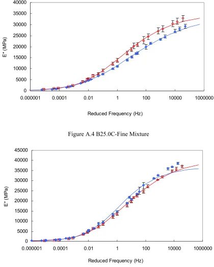
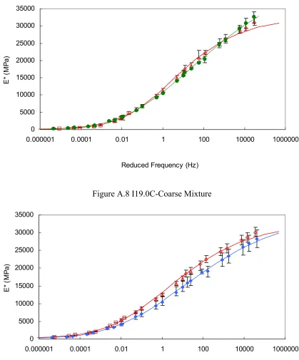
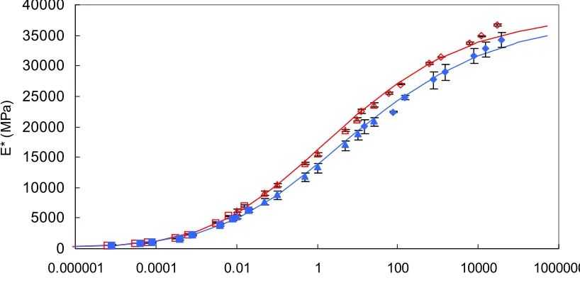
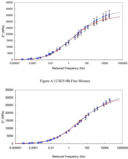
dynamic modulus mastercurves from these analyses are plotted in Figures 5.1 to 5.3 for the
12 mixtures. The data presented in these figures are the average of the three replicates. It can
be observed from these figures that the dynamic modulus mastercurves developed from the
IDT test using the biaxial LVE solution are generally in good agreement with those
factors obtained during the construction of mastercurves were essentially identical for the
axial compression and IDT tests.
Figure 5.1 Dynamic modulus master curves for: (a) S9.5A-Fine mixture; (b) S9.5B-Coarse mixture; (c) S9.5C-Fine mixture; (d) S9.5C-Coarse mixture (Uniaxial data from M. King, 2004)
37
100 1000 10000 100000
1E-06 0.0001 0.01 1 100 10000 1000000
Reduced Frequency (Hz)
E* (M P a ) Uniaxial IDT 100 1000 10000 100000
1E-06 0.0001 0.01 1 100 10000 1000000
Reduced Frequency (Hz)
E* (M P a ) Uniaxial IDT 100 1000 10000 100000
1E-06 0.0001 0.01 1 100 10000 1000000
Reduced Frequency (Hz)
E* (M P a ) Uniaxial IDT 100 1000 10000 100000
1E-06 0.0001 0.01 1 100 10000 1000000
Reduced Frequency (Hz)
38
100 1000 10000 100000
1E-06 0.0001 0.01 1 100 10000 1000000
Reduced Frequency (Hz)
E* ( M P a ) Uniaxial IDT 100 1000 10000 100000
1E-06 0.0001 0.01 1 100 10000 1000000
Reduced Frequency (Hz)
E* (M Pa ) Uniaxial IDT 100 1000 10000 100000
1E-06 0.0001 0.01 1 100 10000 1000000
E* ( M P a ) Uniaxial IDT 100 1000 10000 100000
1E-06 0.0001 0.01 1 100 10000 1000000
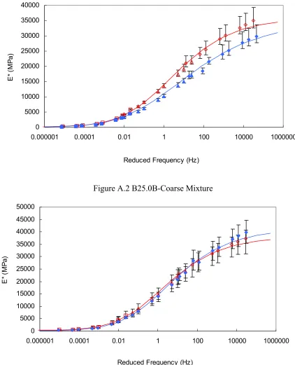
Figure 5.3 Dynamic modulus master curves for: (a) I19.0D-Fine mixture; (b) I19.0D-Coarse mixture; (c) B25.0B-Fine mixture; (d) B25.0B-Coarse mixture (Uniaxial data from M. King, 2004)
39
100 1000 10000 100000
1E-06 0.0001 0.01 1 100 10000 1000000
Reduced Frequency (Hz)
E* (M P a ) Uniaxial IDT 100 1000 10000 100000
1E-06 0.0001 0.01 1 100 10000 1000000
Reduced Frequency (Hz)
E* (M P a ) Uniaxial IDT 100 1000 10000 100000
1E-06 0.0001 0.01 1 100 10000 1000000
Reduced Frequency (Hz)
E* (M P a ) Uniaxial IDT 100 1000 10000 100000
1E-06 0.0001 0.01 1 100 10000 1000000
Reduced Frequency (Hz)
5.1.2 Statistical Analysis
5.1.2.1 Using P-Value
Recognizing that there exists a sample-to-sample variation, a statistical analysis was
conducted using the unequal variance t-test for each mixture at two frequencies for each
testing temperature. In this analysis, all the individual replicates (three from the axial
compression and three from the IDT) were used. The null hypothesis is that the dynamic
modulus from the IDT test is the same as that from the axial compression test. The P-value
was calculated and compared with the critical value of 0.05 to reject or accept the null
hypothesis. The P-value indicates the extent to which a computed test statistic is unusual in
comparison with what would be expected under the null hypothesis. Therefore, in this study a
P-value greater than 0.05 indicates that the dynamic modulus from the IDT test is statistically
the same as that from the axial compression test. The summary of the P-values for 144 tests
(2 frequencies × 3 temperatures × 24 mixtures) is given in Table 5.1. About 19% of the tests indicate that the dynamic modulus from the IDT test is statistically different from the
Table 5.1 Summary of P-Values and Percent Difference in Dynamic Moduli from IDT and Axial Compression Tests
5.1.2.2 Using Percent Difference
In addition to the statistical analysis, % difference was calculated between the
dynamic moduli from the axial compression and IDT tests for 288 combinations of
temperature and frequency (8 frequencies × 3 temperatures × 12 mixes). These values are also summarized in Table 5.1. The comparison of the data in this table and further
investigation of individual test data resulted in several important observations. First, about
70% of the tests had a % difference below 10%. Secondly, although it is not shown in Table
5.1, further investigation of the testing conditions that have high % differences reveals that
most of the high % difference come from 35ºC data due to very small dynamic modulus
values in the denominator of the % difference calculation. Finally, it can be observed in
Table 5.1 that the % difference becomes greater as the NMSA increases. An investigation of
the individual test data revealed the same trend, that is, the variability among the replicates
increases as the NMSA increases. These observations may be related to the ratio of gauge
length to NMSA. Typically, a factor of 3 is recommended to maintain a representative
volume element (RVE). Meeting this requirement is not a problem in the axial compression
test geometry. However, in the IDT tests with a 50.8 mm gauge length, this requirement is
satisfied in the 9.5 and 12.5 mm mixes, but not in the 19.0 and 25.0 mm mixes, resulting in a
9.5 mm 12.5 mm 19.0 mm 25.0 mm
P-value
Less Than 0.05 15% 14% 19% 33% 19%
Greater Than 0.05 85% 86% 81% 67% 81%
% Difference
Less Than 5% 48% 46% 28% 25% 39%
Between 5 & 10% 21% 33% 42% 19% 31%
Between 10 & 20% 21% 21% 26% 19% 22%
Greater Than 20% 10% 0% 4% 38% 8%
higher variability among replicates and a higher % difference in the 19.0 and 25.0 mm mixes.
Another observation made from a detailed data analysis is that, in some replicates of the 25.0
mm mix, a significant difference was found between displacements from the front and back
surfaces of the IDT specimens. These observations suggest that the positions of large
aggregate particles within the gauge length affect the data, and that a larger gauge length is
required for 25.0 mm mixes. These observations are further supported in Chapter 6.
The visual observation of the average mastercurves in Figures 5.1 to 5.3 and further
statistical analyses suggest that the dynamic modulus determined from the IDT test using the
linear viscoelastic solution in Eq. (2-25) is statistically the same as the one measured from
the axial compression test. This observation answers at least a portion of the question raised
earlier regarding the effect of different relationships between the compaction direction and
the direction in which the stress-strain analysis is performed in the axial compression and the
IDT tests. This difference and possibly anisotropy may exist when the axial compression
cylinders and the IDT specimens are compared. However, due to very small strain levels
used in these tests (50 to 80 microstrains), the dynamic modulus test more or less “tickles”
the mastic and does not fully capture the effect of these differences that are mostly related to
the large aggregate orientation.
5.2 Phase Angle
It was observed that the phase angle obtained from axial compression is normally
more rigorous approach. Appendix A contains more phase angle comparisons between IDT
and axial compression tests.
0 5 10 15 20 25 30 35 40
0.000001 0.0001 0.01 1 100 10000 1000000
Reduced Frequency, Hz
P
has
e A
ngl
e
Axial Comp. IDT Horiz. IDT Vert. Average
0 5 10 15 20 25 30 35 40
0.000001 0.0001 0.01 1 100 10000 1000000
Reduced Frequency, Hz
P
has
e A
ng
le
Axial Comp. IDT Horiz. IDT Vert. Average
Figure 5.5 I19.0D-Fine mixture phase angle mastercurves
6. AGGREGATE SIZE EFFECT ON SPECIMEN TO SPECIMEN
VARIATION
In this chapter extensive studies have been made to visually observe and quantify the
effect of aggregate size on the variability of test results. Digital Image Correlation (DIC) was
used to visually observe that effect on the actual strain distribution along both axes of the
specimen, and thus on dynamic modulus. Statistical analysis was used to quantify that effect
for each of the four aggregate sizes, 9.5, 12.5, 19, and 25 mm, tested in this thesis.
6.1 Digital Image Correlation (DIC)
Over the past twenty years advancement in optics, computing power, and general
technology have opened numerous avenues in the research arena. DIC is one sector that has
emerged as a powerful tool for material testing. In simplistic terms, DIC is a non-contact full
field displacement/strain measurement technique. The technique is employed by comparing
a digital image of an initial, undeformed specimen to that of a deformed specimen. The test
setup requires a digital camera, light source, personal computer and software for post testing
analysis.
With LVDT’s, the area of interest must be predefined because the sensors must be
mounted to the test specimen. For example, the vertical and horizontal axes are generally
chosen and analyzed as per the prior discussion. However, with DIC a full field of data is
acquired during testing so there is no limit to the area of interest provided the area of interest
forms a grayscale map for each pixel within the area of interest and compares it with an
original, undeformed image to calculate deformations.
The purpose of this study is to determine the actual strain distribution along the
vertical and horizontal axes of the specimen using DIC for two mixtures with different
NMSA, one being a surface coarse andthe other being a base coarse. The two mixtures are
S 9.5C-Fine and B 25.0C-Fine. In this study “point strain” profiles along a specified gauge
length will be evaluated.
6.1.1 Test Method
6.1.1.1 Test Protocol
As mentioned earlier, the increased technology has allowed for faster acquisition
rates. However, the limiting factor is still the acquisition rate. The camera used for this
testing has a maximum acquisition rate of 0.5 second. Therefore this technology is not yet
capable of collecting cyclical data. For example, with a 0.5 second acquisition rate and a 2
Hz cyclical loading rate would only allow the camera to acquire one point per cycle which in
no way defines the loading and/or displacement curves. Thus a constant crosshead rate
monotonic IDT testing was adopted in this study. A constant crosshead rate of 0.5 inch per
minute was applied to failure of the specimen. This strain rate proved to be suitable to the
6.1.1.2 Testing Equipment
Testing was performed using the same equipment used in dynamic modulus testing.
A National Instruments data acquisition board was used to acquire load and displacement
data from the testing machine. Also, a charge-coupled device (CCD) digital camera
manufactured by Pulnix equipped with a 35-70 mm lens was used in the image acquisition.
The data acquisition board used for image acquisition was distributed by Bitflow. Correlated
Solutions produced the software used to acquire and synchronize the image, load, and
displacement data.
6.1.1.3 Test Setup
The SHRP LGD was used as the loading apparatus in the IDT test. The CCD camera
was mounted and leveled on a tripod at a fixed distance from the specimen. The spacing of
the camera from the specimen was a function of the zoom and physical distance. What is
most important is that the area of interest is as large as possible in the picture’s overall
dimensions. Picture dimensions are measured in pixels and it is desirable to have the best
resolution possible. This is accomplished by minimizing the physical dimension per pixel.
A grayscale map of each pixel is formed thus illustrating the need for many
contrasting points speckled on the specimen surface. The specimen was illuminated using a
fiber optic light source in order to aid in the contrast. The lens used in this study had a
variable aperture that allowed the lens to be adjusted based on the ambient and applied
illumination. Too much light can simply create a solid white image while too little light will
create a solid black image. The process of obtaining the correct amount of light is important
6.1.2 Data Analysis
6.1.2.1 Data Acquisition and Analysis Software
Ram displacements, load cell measurements and images were collected using
software produced by Correlated Solutions. The rate of acquisition was at 0.5 seconds
intervals. Once the images were acquired, post testing analysis software called VIC 2-D was
used to calculate the strain and displacement data. The following sections describe several
key parameters in the analysis process that should be defined before the analysis is done.
6.1.2.2 Area of Interest
A thin rectangular strip was selected along both the vertical and the horizontal axes of
the specimen for analysis. Figures 6.1 and 6.2 illustrate the area of interest selected in both
axes. The width selected was approximately 0.65 inch, which was wide enough to allow the
analysis software to successfully compute “local strain” values, or the strain at any given
point. The width of the strip needed to be minimized so that only behavior along the vertical
and horizontal axes would be observed but it also needed to be wide enough to average the
behavior. A single pixel width would not necessarily provide a general trend across the
diameter of the specimen but rather a jagged relationship between the strain and the radius
Figure 6.1 Vertical area of interest
6.1.2.3 Seed Point
The term “seed point” refers to the point within the area of interest where the
correlation is started. The correlation algorithms use the information from the seed point to
obtain an initial guess for the second point analyzed and continues in this manner until all
points in the area of interest are analyzed. The seed point should be placed in a region where
the least amount of motion occurs during the test. It is easier to correlate the undeformed
image with the deformed image if little movement has occurred between the seed point
locations in each image. Selection of the seed point was consistent for all the horizontal
strips analyzed and for all the vertical strips analyzed. The small box with an X in the middle
in Figures 6.1 and 6.2 illustrate the seed point location for each of the areas of interest that
were analyzed.
6.1.2.4 Strain Calculation
The strain calculation is the most complex portion of this evaluation. The strain must
be evaluated within a small subset of the larger area of interest. The movement of surface is
easily determined but the gauge length that is used is the critical portion. The evaluation is
not as simple as a change in length divided by length approach. The movement observed
must be evaluated in the local region of the point. Advanced mathematical techniques are