1
Wealth accumulation in rotation forestry – failure of the Net Present Value
1
optimization?
2
3
4
Petri P. Kärenlampi 5
6
University of Eastern Finland 7
PO Box 111 8
FIN-80101 Joensuu 9
10
12
tel. +358-50-371 1851 13
fax +358-13-251 4422 14
15 16
17
18
Abstract
19
We investigate wealth accumulation in forestry, assuming that revenues are re-invested. Three
20
different optimization criteria are compared, two of which are based on cash flows, the third
21
financially grounded. Direct optimization of wealth appreciation rate always yields best results.
22
Procedures gained by maximizing internal rate of return are only slightly inferior. With external
23
discounting interest rate, the maximization of net present value yields arbitrary results, with at
24
worst devastating financial consequences.
25
26
Keywords
27
Capital return; real estate; capitalization
28
29
30
2 31
1. Introduction
32
33
We are interested in the accumulation of wealth within the business of forestry. In other words,
34
we are interested in forestry as a financial business. For financial purposes, a variety of
35
economical optimization approaches can be used.
36
37
Most commonly, a discounting interest rate is applied in order to compute the present value of
38
future incomes and expenses (1, 2, 3, 4, 5, 6, 7, 8, 9, 10). The discounting interest may vary
39
over time (11, 12, 13, 14). It has been stated that uncertainty induces declining discount rates
40
along with time (15, 11, 16, 17); however it can be shown that there is an opposite effect on
41
prolongation interest. Risk of destructive events has been considered as a premium to discount
42
interest (18, 19). Evolution of prices, as well as fluctuations in growth and prices, may be added
43
(12, 20). Taxation does contribute, as well as personal financies (21, 22, 23). Imperfect capital
44
market has been addressed (24). A Hamiltonian formulation is available (25, 26). Regardless
45
of other details, financial soundness of any operation significantly depends on the choice of the
46
discounting interest rate.
47
48
We are aware of one method in the determination of profitability in multiannual growth without
49
an external discount rate (27, 28). Sound management is supposed to maximize internal
50
discounting interest (or internal rate of return), harvesting income being discounted to cover
51
initial investments (27, 28). There are a few problems related to this approach: it cannot be
52
applied in the case of zero initial investment, and it does not consider the shape of the yield
53
curve in any way. The latter deficiency is related to the fact that being established on cash-flow
54
basis, the internal interest discounting cannot account for any time-variable capitalization
55
effect.
56
57
The above-mentioned economical optimization criteria have been established on cash-flow
58
basis. Recently, an optimization criterion has been established on financial grounds (29, 30).
59
A representative capital return rate has been produced by integrating a momentary capital
60
return, multiplied by a partition function of capitalization, along time-consequent path within
61
a state space (29). The capitalization has been distributed to operative and non-operative
62
capitalization, and it has been found financially sound forestry practices are dictated by the
63
non-operative capitalization, along with its appreciation rate (30). It is important to note that
3
capitalization can be changed any time by either investing, harvesting, or by selling the real
65
estate, completely or partially. Regarding harvestings, thinning from above may reduce
66
capitalization quickly, as delaying thinnings may increase it. In other words, forest properties
67
can be liquidized at any time, partially or completely, as any other financial asset.
68
69
In this paper, we investigate the effect of objective function on wealth accumulation, assuming
70
that revenues are re-invested. We first present a more general formulation, but later focus in
71
stationary rotation forestry. Stationary rotation forestry here means that the distribution of stand
72
ages does not evolve. This is practically possible if the stand ages are evenly distributed, and
73
the same duration of rotation cycle is applied to stands. Stationary forestry also implies that
74
prices and expenses do not evolve. We are naturally discussing prices and expenses in real
75
terms.
76
77
We apply three different growth models, and three different sets of boundary conditions, the
78
boundary conditions primarily relating to bare land value. We first introduce a basic notation
79
of wealth accumulation, along with an application to rotation forestry. Then, we introduce the
80
above-outlined three different economic criteria (objective functions) for the optimization of
81
forest management. Thirdly, we introduce the three experimental growth models, and
82
investigate wealth accumulation while any of the three economic criteria are followed. Finally,
83
we compare the three different forest economics approaches from the viewpoint of wealth
84
accumulation.
85
86
2. Methods
87
88
21. Wealth accumulation
89
90
Let us first introduce a very basic notation of wealth accumulation:
91
2 2
1 1
2 1 1 ( )
T T
T T
dW
W T W T dt W T W t r t dt dt
(1),92
where W T
1 is wealth at time T1, W T
2 is wealth at time T2, and r is a relative wealth93
increment rate. Provided the time is expressed in years, r becomes the relative annual wealth
94
increment rate. In the absence of withdravals, Eq. (1) can be rewritten
4
2
1
2 1 exp ( )
T
T
W T W T r t dt
(2).
96
97
The above equations describe the total amount of wealth. It possibly should be constituted from
98
stand-level capitalizations, given per unit area. By definition, the expected value capitalization
99
per unit area is
100 0 ( ) p d
(3),101
where ( )p is the probability density function of capitalization. By change of variables we
102
get
103
0 0
( ) d ( ) ( )
p da p a a da da
(4),104
where a is stand age, and is rotation age. The expected value of the increment rate of
105 capitalization is 106 0 ( ) ( )
d d a
p a da
dt dt
(5).107
108
Correspondingly, the momentary expected rate of relative capital return is
109 0 0 0 0 ( , ) ( ) ( ) ( , ) ( , ) ( ) ( ) ( , ) ( ) ( , )
d a t
d p a da p a a t r a t da dt
dt r t
p a a t da p a a t da
(6), 110which can be readily substituted to Eq. (2).
111
112
It is worth noting that in Eq. (6), there is a notation of stand age (a) and a notation of time (t).
113
The probability density of stand age ( )p a could vary as a function of time. However, that would
114
result as a treatment too complicated for the present purposes. Constancy of the stand age
115
distribution is a real possibility if there is an even distribution of stand ages, varying between
116
zero and the rotation age .
117
118
It is indicated in Eq. (6) that the capitalization ( , ) a t , as well as the momentary capital return
119
rate, ( , )r a t are functions of time, in addition to stand age. This would be the case if there
5
would be an appreciation of real estate values, for example, and an eventual appreciation of
121
real estate values might considerably contribute to financial sustainability (30). However, in
122
this paper we discuss forestry in terms of stationary capitalization per unit area. This
123
corresponds to assuming that wood stumpage prices, as well as real estate prices, develop along
124
with general development of prices and expenses. Then, the capital return rate ( )r a corresponds
125
to real return, excluding eventual inflation of prices.
126
127
Now, in the case of constant capitalization per unit area, Eq. (2) becomes
128
2 1 1 2 1 T T r W T e W T (7). 129 130In other words, the expected value of the relative wealth increment rate r is a unique measure 131
of wealth accumulation, regardless of the time horizon, and it is given by
132 0 0 ( ) ( ) d a da dt r a da
(8). 133 13422. Objective functions to be compared
135
136
Probably the most commonly used objective function used in forestry optimizations is
137
maximization of net present value of future revenues and expenses (1, 2, 3, 4, 5, 6, 7, 8, 9, 10):
138 0 0 1 ( ) 1 it t i
NPV R t e dt
e
(9), 139where R(t) corresponds to net proceeds at time t, i is discounting interest rate, and again is
140
rotation age. The last factor after the integral corresponds to discounting of further growth
141
cycles, each of rotation age .
142
143
A significant problem in Eq. (9) is that it contains the external discount rate i. The discount rate
144
is external in the sense that it is unrelated to the capital return within the growth process, and
145
consequently subject to arbitrary changes. Another issue in Eq. (9) is that it does not consider
146
the shape of the yield curve in any way. In other words, Eq. (9) discusses revenue on cash basis,
147
instead of financial grounds.
6 149
The problem of arbitrary external interest has been resolved by maximizing an internal rate of
150
return. As introduced by Newman (28, 27), it is determined for a period of duration according
151
to the criterion
152
0
( ) ot 0
R t e dt
(10).153
The general form of Eq. (10) does not appear to make sense at first glance. However, the
154
Equation makes complete sense provided negative net proceeds appear in the beginning of the
155
rotation, and positive net proceeds are generated by the end of the growth cycle. It is sometimes
156
stated that maximizing the internal rate of return would not consider any bare land value. Such
157
a statement however is incorrect. Eq. (10) considers one single rotation, whereas Eq. (9) refers
158
to maximization of long-term discounted proceeds. Optimization of one single rotation
159
possibly should consider purchase of bare land at the beginning, and sales of it at the end. Even
160
if actual real estate transaction would not be implemented, the purchase price should be
161
considered as an opportunity cost of not selling the bare land in the beginning. By the end of
162
the single rotation to be optimized, the bare land constitutes a saleable asset.
163
164
Evidently, a third objective function to be compared from the viewpoint of wealth
165
accumulation should be maximization of the expected value of the relative wealth increment
166
rate r , given in Eq. (8). Such an objective function has been recently derived in terms of a 167
state-space approach (29). It might be considered trivial that this criterion is superior from the
168
viewpoint of wealth accumulation, considering that it has been derived as the unique measure
169
of wealth accumulation rate at Eqs. (1…7). However, recent discussion has indicated that this
170
is considered far from trivial. Regardless of the eventual triviality, it is of interest how much
171
inferior objective functions (9) and (10) might be, in comparison to (8).
172
173
174
23. Forest growth models applied
175
176
231. Volumetric growth model for pine
177
178
As the first practical example, we consider a recently introduced (9) yield function, applicable
179
to average pine stands in Northern Sweden. A volumetric growth function is
7 181
/95
2.8967580.14* 1 6.3582 t
V t (11).
182
183
The application introduced by Gong and Löfgren [9] assumes a volumetric stumpage price of
184
250 SEK/m3 and an initial investment of 6000 SEK/ha. The maximum sustained volumetric
185
yield rotation is 95 years, corresponding to that duration of time that gives the greatest average
186
annual growth [9]. A 3% discount interest applied in Eq. (9) yields an optimal rotation age of
187
52 years (Gong and Löfgren 2016).
188
189
232. Value growth model for pine
190
191
Eq. (11) does not consider any variation of the volumetric stumpage price. In other words, the
192
value growth corresponds to volumetric growth, multiplied by a constant. That may be an
193
unrealistic assumption, for a variety of reasons, including harvesting expenses as well as
194
industrial use of the crop. In order to release this assumption, Gong and Löfgren [9] established
195
an age-dependent price function
196
197
104.63*
29
0.2602p t t (12).
198
199
We here apply Eq. (12), for t>29, in addition to Eq. (11), in order to establish another version
200
of the practical forestry example. Maximum sustainable value yield is gained at 130 years of
201
rotation. A 3% discount interest applied in Eq. (9) yields an optimal rotation age of 62 years
202
[9].
203
204
205
206
233. Value growth model for spruce
207
208
The third empirical model describes fertile spruce forests with natural regeneration. We will
209
again assume a constant stand age distribution, as in Eq. (8), but now the stand age does not
210
refer to the age of trees, but to time elapsed after the latest regeneration harvesting of any stand.
211
We apply the empirical model of Bollandsås et al. (31, 32), and parametrize it with reference
212
to a recently introduced stationary state (33, 30).
8 214
We define any regeneration harvesting with respect to a natural stationary state (33, 30). In
215
particular, we introduce a diameter-limit cutting to breast height diameter 25 cm, and adjust
216
the number of remaining trees within any diameter class below 25 cm to the number of trees in
217
the natural stationary state (33, 30). Then, we allow any stand to develop according to the
218
empirical model by Bollandsås et al. [31, 32], until a particular rotation age, where another
219
regeneration harvesting is assumed to occur. We parametrize the model with site fertility index
220
20, which corresponds to dominant height in meters for an even-aged stand of 40 years of age
221
[31, 32].
222
223
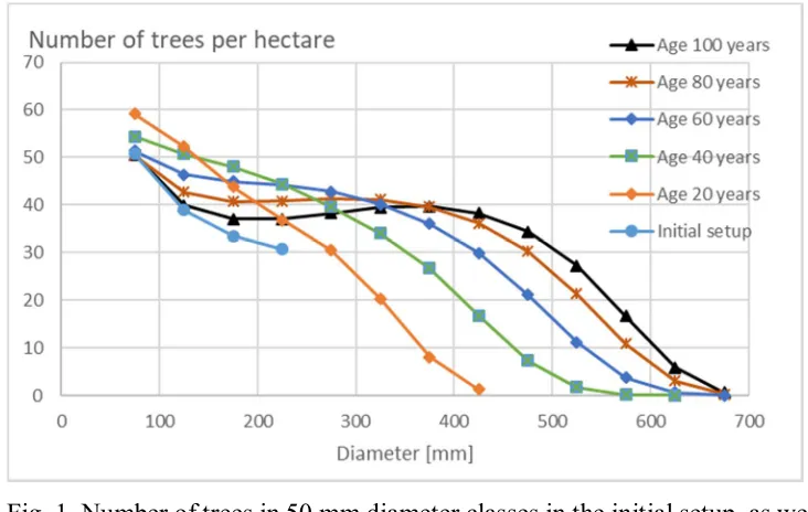
The number of trees per hectare in different diameter classes, according to the model described
224
above, is shown in Fig. 1. The initial setup naturally contains only trees of diameter less than
225
250 mm. The number of trees in any diameter class, except the smallest, is smaller than in
226
developed stages. A consequence is that the regeneration harvesting not only contains
227
diameter-limit cutting, but also some thinning of smaller trees.
228
229
On the basis of the number of trees per hectare, we clarify the volumetric amount of two
230
assortments, pulpwood and sawlogs, according to an appendix given by of Rämö and Tahvonen
231
[34, 35]. The monetary value of the assortment volumes is clarified according to stumpage
232
prices given by Rämö and Tahvonen [34]. In the initial setup, the number of trees (breast-height
233
diameter at least 50 mm) per hectare is 154. The basal area is 2.72 m2/ha, and the combined
234
volume of the assortments 18.5 m3/ha. The stumpage value of the trees in the initial setup is
235
670 Eur/ha.
236
9 238
Fig. 1. Number of trees in 50 mm diameter classes in the initial setup, as well as later stages of
239
stand development, according to the spruce growth model (31, 32, 33, 30). Stand age refers to
240
lime elapsed after the latest regeneration harvesting.
241
242
24. Analytical procedures
243
244
For any of the three growth models (Eq. (11), and (11) combined with (12), and (31, 32, 33,
245
30), we optimize the rotation age according to any of the three different objective functions
246
given in Eqs. (9), (10) and (8). Maximization of the net present value of proceeds according to
247
Eq. (9) requires an external discount interest rate. We adopt three different rates, 2%, 3% and
248
4%. Maximization of the internal rate of return according to Eq. (10), as well as the expected
249
value of capital return according to Eq. (8) require a bare land value, as an opportunity cost in
250
Eq. (10) and as a part of the applied capitalization in Eq. (8). We apply three different bare land
251
values: zero, a moderate, and a high bare land value. In the case of pine stand models with a
252
regeneration expense, the moderate value equals half of the regeneration expense, and the high
253
value two times the regeneration expense. In the case of the spruce model with natural
254
regeneration, the moderate value is 70% of the value of trees in the initial setup, and the high
255
value 300% of the value of trees in the initial setup. Since we are discussing stationary forestry,
256
we do not consider any appreciation of the real estate prices.
257
258
After determining the optimal rotation age for three different growth models, using the three
259
objective functions, we find out what kind of expected value of relative wealth increment rate
10
those rotation ages yield according to Eq. (8). Again, this is done using the three different bare
261
land values as explained above. Eq. (8) of course can be substituted to Eq. (7) or to Eq. (2).
262
263
In order to apply Eq. (8), we need an amortizations schedule for any eventual initial investment.
264
We choose to make a one-time amortization at the end of any rotation, simultaneously as the
265
final proceeds are gained. A consequence is that there is no amortization of initial investment
266
affecting the denominator of Eq. (8); the investment expense contributes to the capitalization
267
during the entire rotation. On the other hand, the change of capitalization during the rotation,
268
appearing in the numerator of Eq. (8), is net of regeneration expense.
269
270
271
3. Results
272
273
31. Pine volumetric growth model
274
275
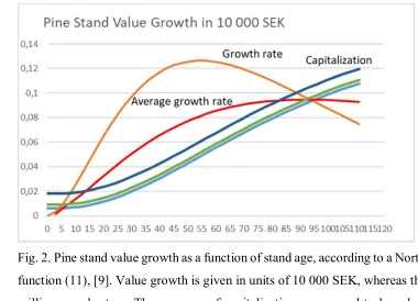
Let us first plot the momentary capitalization ( ) a , as well as the increment rate of momentary
276
capitalizationd
da
as a function of stand age a in Fig. 2. The result is an outcome of the growth
277
model only and does not depend on the objective function applied. The increment rate of
278
capitalization does not depend on the bare land value, whereas the capitalization itself does.
279
We find that the average increment rate of capitalization reaches the momentary increment rate
280
at stand age 95 years, which corresponds to the rotation age of maximum sustainable
281
volumetric yield.
282
11 284
Fig. 2. Pine stand value growth as a function of stand age, according to a North-Swedish growth
285
function (11), [9]. Value growth is given in units of 10 000 SEK, whereas the capitalization in
286
millions per hectare. Three curves of capitalization correspond to bare land values 0, 3000
287
SEK/ha and 12 000 SEK/ha.
288
289
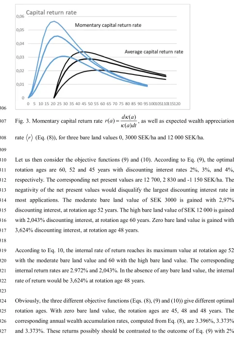
Let us then plot the momentary capital return rate ( ) ( ) ( )
d a r a
a dt
as a function of stand age a,
290
and the expected value of the wealth appreciation rate r (Eq. (8)) as a function of rotation
291
age . These both are drawn in Fig. 3. We find that for any of the three bare land values, the
292
expected value of the wealth appreciation rate reaches the momentary value at the maximum
293
value of the former. The regeneration expense, as well as the bare land value taken as constants,
294
the actual wealth appreciation rate depends on the rotation age according to Eq. (8). The
295
optimal rotation ages for bare land values 0, 3000 SEK/ha and 12 000 SEK/ha are 45, 48 and
296
56 years, corresponding to wealth appreciation rates to 3.396%, 2.877% and 2.047% per
297
annum.
298
299
It is worth noting that in Fig. 3, the momentary capital return rate is given as a function of stand
300
age a, without any reference to any particular rotation age . We chose to make a one-time
301
amortization at the end of any rotation, the momentary capital return rate does not contain any
302
amortization. On the other hand, the wealth appreciation rate r is given as a function of
303
rotation age, and correspondingly the amortization contributes to it. That is why r first
304
becomes nonnegative at rotation age of 21 years.
12 306
Fig. 3. Momentary capital return rate ( ) ( ) ( )
d a r a
a dt
, as well as expected wealth appreciation
307
rate r (Eq. (8)), for three bare land values 0, 3000 SEK/ha and 12 000 SEK/ha.
308
309
Let us then consider the objective functions (9) and (10). According to Eq. (9), the optimal
310
rotation ages are 60, 52 and 45 years with discounting interest rates 2%, 3%, and 4%,
311
respectively. The corresponding net present values are 12 700, 2 830 and -1 150 SEK/ha. The
312
negativity of the net present values would disqualify the largest discounting interest rate in
313
most applications. The moderate bare land value of SEK 3000 is gained with 2,97%
314
discounting interest, at rotation age 52 years. The high bare land value of SEK 12 000 is gained
315
with 2,043% discounting interest, at rotation age 60 years. Zero bare land value is gained with
316
3,624% discounting interest, at rotation age 48 years.
317
318
According to Eq. 10, the internal rate of return reaches its maximum value at rotation age 52
319
with the moderate bare land value and 60 with the high bare land value. The corresponding
320
internal return rates are 2.972% and 2,043%. In the absence of any bare land value, the internal
321
rate of return would be 3,624% at rotation age 48 years.
322
323
Obviously, the three different objective functions (Eqs. (8), (9) and (10)) give different optimal
324
rotation ages. With zero bare land value, the rotation ages are 45, 48 and 48 years. The
325
corresponding annual wealth accumulation rates, computed from Eq. (8), are 3.396%, 3.373%
326
and 3.373%. These returns possibly should be contrasted to the outcome of Eq. (9) with 2%
13
and 3% discounting interests, which would give optimal rotation ages 60 and 52 years. These
328
rotation ages, according to Eq. (8), give capital appreciation rates 3,075% and 3,300%,
329
respectively.
330
331
With the moderate bare land value of 3000 SEK/ha, the rotation ages are 48, 52 and 52 years.
332
The corresponding annual wealth accumulation rates, computed from Eq. (8), are 2.877%,
333
2.857% and 2.857%. These returns possibly should be contrasted to the outcome of Eq. (9)
334
with 2% and 3% discounting interests, which again give optimal rotation ages 60 and 52 years.
335
These rotation ages, according to Eq. (8) but now with the bare land value 3000 SEK/ha, give
336
capital appreciation rates 2,726% and 2.857%, respectively.
337
338
With the high bare land value of 12 000 SEK/ha, the rotation ages are 56, 60 and 60 years. The
339
corresponding annual wealth accumulation rates, computed from Eq. (8), are 2.047%, 2.035%
340
and 2.035%. These returns again should be contrasted to the outcome of Eq. (9) with 2% and
341
3% discounting interests, which again give optimal rotation ages 60 and 52 years. These
342
rotation ages, according to Eq. (8) but now with the bare land value 12 000 SEK/ha, give capital
343
appreciation rates 2,035% and 2.037%, respectively.
344
345
We find that with this growth model, Eq. (10) gives rotation ages and wealth appreciation rates
346
rather close to the optimum. Since the outcome of Eq. (9) depends on the discounting interest
347
rate, the results vary. In the case of zero and moderate bare land values, the outcome with 2%
348
discounting interest differs from the optimal. In the of the high bare land value, the outcome of
349
Eq. (9) differs only slightly from the optimum, with any of the two discounting interest rates.
350
351
Rather interestingly, the results from Eqs. (9) and (10), regarding rotation time and wealth
352
appreciation rate, are identical provided the discounting interest rate in Eq. (9) is adjusted to
353
result in any known bare land value as a net present value of future proceeds. The adjusted
354
discounting interest rate in Eq. (9) is the same as the internal rate of return in Eq. (10). This
355
leads us to suspect that the two objective functions possibly are identical.
356
357
358
359
360
14
32. Pine value growth model
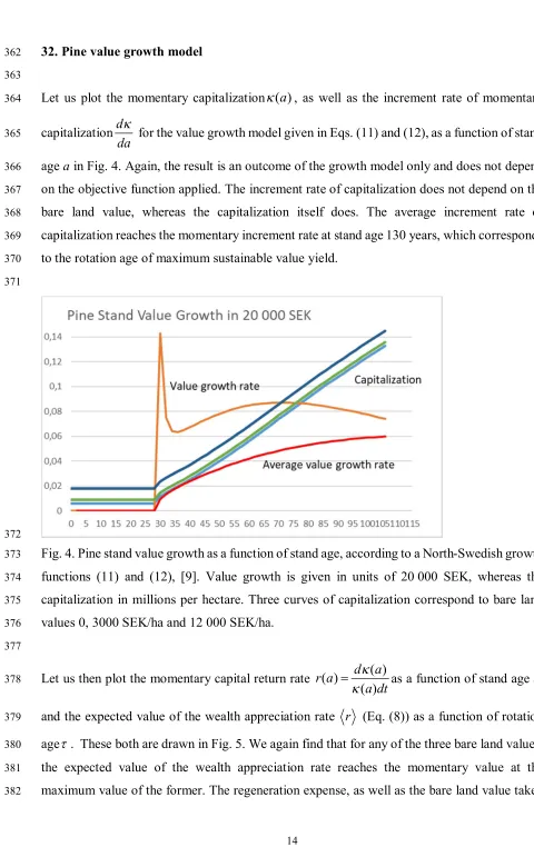
362
363
Let us plot the momentary capitalization ( ) a , as well as the increment rate of momentary
364
capitalizationd
da
for the value growth model given in Eqs. (11) and (12), as a function of stand
365
age a in Fig. 4. Again, the result is an outcome of the growth model only and does not depend
366
on the objective function applied. The increment rate of capitalization does not depend on the
367
bare land value, whereas the capitalization itself does. The average increment rate of
368
capitalization reaches the momentary increment rate at stand age 130 years, which corresponds
369
to the rotation age of maximum sustainable value yield.
370
371
372
Fig. 4. Pine stand value growth as a function of stand age, according to a North-Swedish growth
373
functions (11) and (12), [9]. Value growth is given in units of 20 000 SEK, whereas the
374
capitalization in millions per hectare. Three curves of capitalization correspond to bare land
375
values 0, 3000 SEK/ha and 12 000 SEK/ha.
376
377
Let us then plot the momentary capital return rate ( ) ( ) ( )
d a r a
a dt
as a function of stand age a,
378
and the expected value of the wealth appreciation rate r (Eq. (8)) as a function of rotation
379
age . These both are drawn in Fig. 5. We again find that for any of the three bare land values,
380
the expected value of the wealth appreciation rate reaches the momentary value at the
381
maximum value of the former. The regeneration expense, as well as the bare land value taken
15
as constant, the actual wealth appreciation rate depends on the rotation age according to Eq.
383
(8). The optimal rotation ages for bare land values 0, 3000 SEK/ha and 12 000 SEK/ha are 49,
384
54 and 63 years, corresponding to wealth appreciation rates to 4.034%, 3.347% and 2.354%
385
per annum.
386
387
It is worth noting that in Fig. 5, the momentary capital return rate is given as a function of stand
388
age a, without any reference to any particular rotation age . We chose to make a one-time
389
amortization at the end of any rotation, so the momentary capital return rate does not contain
390
any amortization. On the other hand, the wealth appreciation rate r is given as a function of
391
rotation age, and correspondingly the amortization contributes to it. That is why r first
392
becomes nonnegative at rotation age of 31 years.
393
394
395
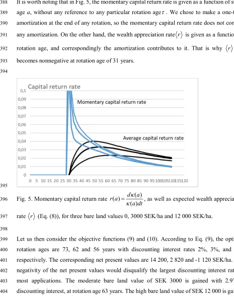
Fig. 5. Momentary capital return rate ( ) ( ) ( )
d a r a
a dt
, as well as expected wealth appreciation
396
rate r (Eq. (8)), for three bare land values 0, 3000 SEK/ha and 12 000 SEK/ha.
397
398
Let us then consider the objective functions (9) and (10). According to Eq. (9), the optimal
399
rotation ages are 73, 62 and 56 years with discounting interest rates 2%, 3%, and 4%,
400
respectively. The corresponding net present values are 14 200, 2 820 and -1 120 SEK/ha. The
401
negativity of the net present values would disqualify the largest discounting interest rate in
402
most applications. The moderate bare land value of SEK 3000 is gained with 2.972%
403
discounting interest, at rotation age 63 years. The high bare land value of SEK 12 000 is gained
16
with 2.126% discounting interest, at rotation age 71 years. Zero bare land value is gained with
405
3.549% discounting interest, at rotation age 58 years.
406
407
According to Eq. 10, the internal rate of return reaches its maximum value at rotation age 63
408
with the moderate bare land value and 71 with the high bare land value. The corresponding
409
internal return rates are 2.972% and 2.126%, respectively. In the absence of any bare land
410
value, the internal rate of return would be 3.549% at rotation age 58 years.
411
412
Obviously, the three different objective functions (Eqs. (8), (9) and (10)) shall give different
413
optimal rotation ages. With zero bare land value, the rotation ages are 49, 58 and 58 years. The
414
corresponding annual wealth accumulation rates, computed from Eq. (8), are 4.034%, 3.859%
415
and 3.859%. With the moderate bare land value of 3000 SEK/ha, the rotation ages are 54, 63
416
and 63 years. The corresponding annual wealth accumulation rates, computed from Eq. (8), are
417
3.347%, 3.222% and 3.222%. With the high bare land value of 12 000 SEK/ha, the rotation
418
ages are 63, 71 and 71 years. The corresponding annual wealth accumulation rates, computed
419
from Eq. (8), are 2.354%, 2.308% and 2.308%.
420
421
Interestingly, the results based on Eqs. (9) and (10) are again identical. This is the case provided
422
the discounting interest used in Eq. (9) is calibrated to gain the same bare land value as is used
423
as input variable in Eq. (10). The situation is different if arbitrary discounting interests are used
424
in Eq. (9). With 2% and 3% discounting interests, the optimal rotation ages would be 73 and
425
62 years, respectively. According to Eq. (8), these rotation ages would yield capital
426
appreciation rates 3.263% and 3.713% for zero bare land value, 2.948% and 3.244% for
427
moderate bare land value, and 2.286% and 2.353% for the high bare land value. In the case of
428
zero and moderate bare land values, the outcome with 2% discounting interest again differs
429
from the optimal, this time more severely than in the case of the volumetric growth model
430
discussed above.
431
432
33. Spruce value growth model
433
434
Let us plot the momentary capitalization ( ) a , as well as the increment rate of momentary
435
capitalizationd
da
for the spruce value growth model (31, 32, 33, 30), as a function of stand age
436
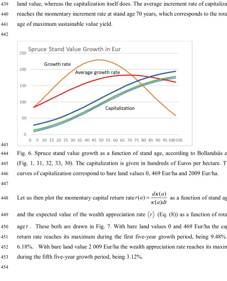
a in Fig. 6. Again, the result is an outcome of the growth model only and does not depend on
17
the objective function applied. The increment rate of capitalization does not depend on the bare
438
land value, whereas the capitalization itself does. The average increment rate of capitalization
439
reaches the momentary increment rate at stand age 70 years, which corresponds to the rotation
440
age of maximum sustainable value yield.
441
442
443
Fig. 6. Spruce stand value growth as a function of stand age, according to Bollandsås et al.
444
(Fig. 1, 31, 32, 33, 30). The capitalization is given in hundreds of Euros per hectare. Three
445
curves of capitalization correspond to bare land values 0, 469 Eur/ha and 2009 Eur/ha.
446
447
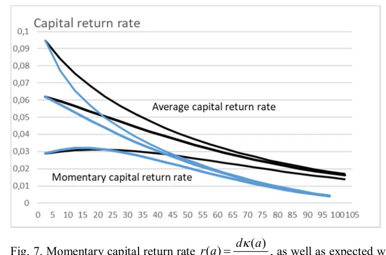
Let us then plot the momentary capital return rate ( ) ( ) ( )
d a r a
a dt
as a function of stand age a,
448
and the expected value of the wealth appreciation rate r (Eq. (8)) as a function of rotation
449
age . These both are drawn in Fig. 7. With bare land values 0 and 469 Eur/ha the capital
450
return rate reaches its maximum during the first five-year growth period, being 9.48% and
451
6.18%. With bare land value 2 009 Eur/ha the wealth appreciation rate reaches its maximum
452
during the fifth five-year growth period, being 3.12%.
453
18 455
Fig. 7. Momentary capital return rate ( ) ( ) ( )
d a r a
a dt
, as well as expected wealth appreciation
456
rate r (Eq. (8)), for three bare land values 0, 469 Eur/ha and 2 009 Eur/ha.
457
458
Let us then consider the objective functions (9) and (10). According to Eq. (9), the optimal
459
rotation ages are 40, 25 and 10 years with discounting interest rates 2%, 3%, and 4%,
460
respectively. The corresponding net present values of the initial setup (bare land and trees
461
standing after the regeneration harvesting) are 5062, 2821 and 1905 Eur/ha. The moderate
462
initial setup value of Eur 1139 is gained with 6.24% discounting interest, at rotation age 5
463
years. The high initial setup value of Eur 2679 is gained with 3.11% discounting interest, at
464
rotation age 25 years. Initial setup value consisting only of trees remaining after the
465
regeneration cutting is gained with 9.68% discounting interest, at rotation age 5 years.
466
467
According to Eq. 10, the internal rate of return reaches its maximum value at rotation age 5
468
with the moderate bare land value and 25 with the high bare land value. The corresponding
469
internal return rates are 6.24% and 3.11%, respectively. In the absence of any bare land value,
470
the internal rate of return would be 9.68% at rotation age 5 years.
471
472
Again, the results based on Eqs. (9) and (10) are identical, provided the discounting interest in
473
Eq. (9) is calibrated to produce a known net present value for the initial setup. In the case of
474
this spruce growth model, also direct optimization according to Eq. (8) gives the same rotation
475
times. Internal rates of return resulting from Eq. (10) slightly differ from wealth accumulation
19
rates coming from Eq. (8), the former Equation neglecting the shape of the yield curve, whereas
477
Eq. (8) does not. The discounting interest rates needed in Eq. (9) to produce known initial
478
setup values as net present values are the same as the internal return rates in Eq. (8).
479
480
The economic views diverge if arbitrary discounting interests are used in Eq. (9). With 2%, 3%
481
and 4% discounting interests, the optimal rotation ages would be 40, 25 and 10 years,
482
respectively. According to Eq. (8), these rotation ages would yield capital appreciation rates
483
4.76%, 6.21% and 8.41% for zero bare land value, 4.16%, 5.04% and 5.92% for moderate bare
484
land value, and 2.94%, 3.12% and 3.00% for the high bare land value.
485
486
487
4. Discussion
488
489
Two of the objective functions discussed above have yielded financially satisfactory results,
490
whereas the third is clearly inferior. However, the inferior method of maximization of net
491
present value appear to yield numerical results identical to those of internal rate of return,
492
provided that the discounting interest in Eq. (9) is calibrated to yield an appropriate bare land
493
value. This raises a question whether the two objective functions are identical with the
494
mentioned boundary condition. We can readily rewrite Eq. (10) for the special case where there
495
are nonzero net proceeds a two time instants: at the beginning of each growth cycle, and at the
496
end of the growth cycle. In the beginning, there is an initial investment I and a purchase
497
expense for the bare land B. At the end of the cycle, there is harvesting revenue H, and sales
498
proceeds for the bare land B. Then, Eq. (10) can be rewritten as
499
RB e
o
IB
0 (13).500
501
Resolving the bare land value yields
502
o
1 1o
B Re I
e
(14).
503
Eq. (12) however is the same as Eq. (9), with the same boundary conditions. One can readily
504
show that the equality applies to any schedule of proceeds where a resource is occupied at the
505
beginning of a period and released at the end.
506
20
Eqs. (13) and (14) demonstrate that two of the above-discussed objective functions are the
508
same, provided the discounting interest rate in Eq. (9) is adjusted to yield an appropriate bare
509
land value. Then, one must ask how can one clarify what is an appropriate bare land value? In
510
the mind of the Author, this is not too difficult. There is bare forest land available in the real
511
estate market. There also are young plantations on the market, and the bare land value is
512
achievable by deducting their regeneration expense. On the other hand, there is no reliable way
513
of determining a valid discounting interest rate, apart from the calibration to yield a valid bare
514
land value. No market interest rate can be selected for the discounting interest; at the time of
515
writing, mortgage interest rates within the Eurozone vary 1%...2%, but an opportunity cost for
516
neglected alternative investments easily becomes 6%...9%. The range is far too wide.
517
518
In a few cases, the wealth appreciation rate is not very sensitive to the objective function
519
selected. However, there are rather sensitive cases. Fig. 8 shows wealth accumulation within
520
the value growth model described in Eqs. (11) and (12), for a period of 70 years, in the absence
521
of any bare land value. We find that there are rather significant differences between the
522
different objective functions. Direct maximization of Eq. (8) results as a rotation age of 49
523
years. Maximization of internal rate of return according to Eq. (10) results as rotation age 58
524
years. Net present value maximization according to Eq. (9) results as rotation ages 73 and 62
525
years, with 2% and 3% discounting interest, respectively. In Fig. 8, wealth accumulation is
526
only slightly suboptimal if rotation age is determined either with Eq. (10) or with Eq. (9) with
527
discounting interest rate 3%. However, with discounting interest 2%, Eq. (9) yields clearly
528
inferior results.
529
530
21
Fig. 8. Wealth accumulation as a function of time (in years) for the value growth model
532
introduced in Eqs. (11) and (12), with bare land value 0 SEK/ha.
533
534
Fig. 9 shows wealth accumulation within the value growth model described in Eqs. (11) and
535
(12), for a period of 70 years, for the moderate bare land value 3000 SEK/ha. We find that there
536
again are rather significant differences between the different objective functions, even if
537
somewhat less than in Fig. 8. Direct maximization of Eq. (8) results as a rotation age of 54
538
years. Maximization of internal rate of return according to Eq. (10) results as rotation age 63
539
years. Net present value maximization according to Eq. (9) results as rotation ages 73 and 62
540
years, with 2% and 3% discounting interest, respectively. We find from Fig. 9 that Eq. (9) with
541
3% discounting interest yields a slightly greater wealth accumulation rate than Eq. (10). This
542
is naturally accidental. The 3% discounting rate in Eq. (9) being selected arbitrarily, it happens
543
to result in one year younger rotation age in the case of Fig. 9. Again, Eq. (9) with discounting
544
interest 2%, yields clearly inferior results.
545
546
547
Fig. 9. Wealth accumulation as a function of time (in years) for the value growth model
548
introduced in Eqs. (11) and (12), with moderate bare land value 3000 SEK/ha. The dotted line
549
corresponds to the internal rate of return optimization according to Eq. (10).
550
551
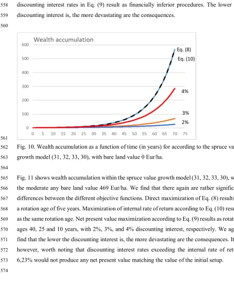
Fig. 10 shows wealth accumulation within the spruce value growth model (31, 32, 33, 30), in
552
the absence of any bare land value. We find that there are rather significant differences between
553
the different objective functions. Direct maximization of Eq. (8) results as a rotation age of five
554
years. Maximization of internal rate of return according to Eq. (10) results as the same rotation
22
age. Net present value maximization according to Eq. (9) results as rotation ages 40, 25 and 10
556
years, with 2%, 3%, and 4% discounting interest, respectively. We find that all these three
557
discounting interest rates in Eq. (9) result as financially inferior procedures. The lower the
558
discounting interest is, the more devastating are the consequences.
559
560
561
Fig. 10. Wealth accumulation as a function of time (in years) for according to the spruce value
562
growth model (31, 32, 33, 30), with bare land value 0 Eur/ha.
563
564
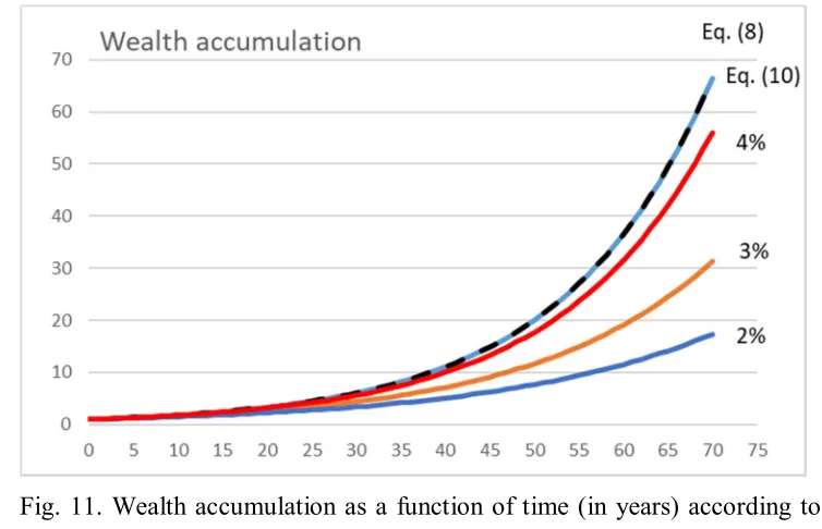
Fig. 11 shows wealth accumulation within the spruce value growth model (31, 32, 33, 30), with
565
the moderate any bare land value 469 Eur/ha. We find that there again are rather significant
566
differences between the different objective functions. Direct maximization of Eq. (8) results as
567
a rotation age of five years. Maximization of internal rate of return according to Eq. (10) results
568
as the same rotation age. Net present value maximization according to Eq. (9) results as rotation
569
ages 40, 25 and 10 years, with 2%, 3%, and 4% discounting interest, respectively. We again
570
find that the lower the discounting interest is, the more devastating are the consequences. It is,
571
however, worth noting that discounting interest rates exceeding the internal rate of return
572
6,23% would not produce any net present value matching the value of the initial setup.
573
23 575
Fig. 11. Wealth accumulation as a function of time (in years) according to the spruce value
576
growth model (31, 32, 33, 30), with moderate bare land value 469 Eur/ha.
577
578
It is of interest to consider why the maximization of the internal rate of return according to Eq.
579
(10) yields wealth appreciation rates lower than direct maximization of Eq. (8). The reason
580
naturally is that the IRR is determined on the basis of cash proceeds and neglects the details of
581
the yield curve. The details of the yield curve however do contribute to the wealth accumulation
582
rate. Regardless of this, maximizing the internal rate of return, in general, does not lead to any
583
large deviation from financially optimal management procedures (Figs. 8, 9, 10 and 11).
584
585
Unlike the internal rate of return, maximization of net present value with external discounting
586
interest rate does induce large deviations from financially optimal management (Figs. 8, 9, 10
587
and 11). However, different discounting interest rates differ. There always is a discounting
588
interest rate where maximizing the net present value becomes equal to maximizing the internal
589
rate of return. However, arbitrarily adopting an external discounting interest leads to highly
590
variable and at worst devastating financial consequences (Figs. 8, 9, 10 and 11). This also
591
applies to discounting interest rates commonly utilized in net present value computations in
592
forestry [36, 34, 37, 38, 39, 40].
593
594
It is worth noting that a 3% discounting rate in Eq. (9), relatively commonly used in forestry
595
(37, 38, Sinha et al., 2017), performs relatively well in the pine growth models discussed above
596
(Figs. 8 and 9), but produces clearly inferior results in the case of the spruce value growth
597
model (Figs. 10 and 11).
24 599
In this paper, we have been discussing stationary rotation forestry. In other words, stand ages
600
have been assumed to be evenly distributed. Prices and expenses have been treated as constants
601
in real terms. It has been recently shown that an eventually appreciating real estate price
602
possibly dictates financially sustainable management practices (30). It would be of interest to
603
investigate such an effect on the performance of the different objective functions.
604
605
606
Acknowledgment
607
608
The Author does not have any particular interest to declare in relation to this paper.
609
610
References
611
612
1. Faustmann, M., 1849. Berechnung des Wertes welchen Waldboden sowie noch nicht
613
haubare Holzbestande fur die Waldwirtschaftbesitzen. Allg Forst- und Jagdz, Dec, 440–455.
614
(On the determination of the value which forestland and immature stands pose for forestry.
615
Reprinted in Journal of Forest Economics 1:7–44 (1995).)
616
2. Pearse, P.H., 1967. The optimum forest rotation. Forestry Chronicle, 43(2), 178-195.
617
3. Samuelson, P. A., 1976. Economics of forestry in an evolving society. Economic Inquiry,
618
14, 466–492.
619
4. Yin, R., Newman, D.H., 1995. Optimal timber rotations with evolving prices and costs
620
revisited. Forest Science, Volume 41(3), 477-490.
621
5. Deegen, P., Hostettler, M., Navarro, G.A., 2011. The Faustmann model as a model for a
622
forestry of prices. Eur. J. Forest Res. 130, 353.
623
6. Campbell, H., 1999. Economics of the Forest - UQ eSpace
624
https://espace.library.uq.edu.au/view/UQ:11074/DP265Oct99.pdf
625
7. Nyyssönen, A., 1999. Kiertoaikamalli Suomen metsätaloudessa. Metsätieteen
626
aikakauskirja 1999(3), 540-543.
627
8. Tahvonen, O., 2016. Economics of rotation and thinning revisited: the optimality of
628
clearcuts versus continuous cover forestry. Forest Policy and Economics 62, 88-94.
629
9. Gong, P., Löfgren, K.-G., 2016. Could the Faustmann model have an interior minimum
630
solution? Journal of Forest Economics 24, 123-129.
25
10. Abdallah, S.B., Lasserre, P., 2017. Forest land value and rotation with an alternative land
632
use. Journal of Forest Economics 29, 118–127.
633
11. Price, C., 2011. Optimal rotation with declining discount rate. J. Forest Economics 17,
634
307-318.
635
12. Buongiorno, J., Zhou, M., 2011. Further generalization of Faustmann’s formula for
636
stochastic interest rates. J. Forest Economics 17, 284-257.
637
13. Brazee, R.J., 2017. Impacts of declining discount rates on optimal harvest age and land
638
expectation values. J. Forest Economics, https://doi.org/10.1016/j.jfe.2017.06.002.
639
14. Price, C., 2017a. Optimal rotation with negative discount rates: completing the picture. J.
640
For. Econ. 29, 87-93.
641
15. Groom, P., Hepburn, C., Koundouri, P., Pearce, D., 2005. Discounting the future: the long
642
and the short of it. Environmental and Resource Economics, 32 (2005), pp. 445-493.
643
16. Hepburn C.J., Koundouri P., 2007. Recent advances in discounting: implications for forest
644
economics. J For Econ 13(2-3):169–189.
645
17. Price, C., 2017b. Declining discount rate and the social cost of carbon: forestry
646
consequences, J. For. Econ. ISSN 1104-6899, https://doi.org/10.1016/j.jfe.2017.05.003.
647
(http://www.sciencedirect.com/science/article/pii/S1104689916300988)
648
18. Loisel, P., 2011. Faustmann rotation and population dynamics in the presence of a risk of
649
destructive events. J. Forest Economics 17, 235-247,
650
19. Hyytiäinen, K., Haight, R.G., 2010. Evaluation of forest management systems under risk
651
of wildfire. Eur. J. Forest Res. 129, 909.
652
20. Yin, R. and Newman, D., 1997. When to cut a stand of trees?. Natural Resource
653
Modeling 10, 251–261.
654
21. Koskela, E., Alvarez, L.H.R., 2004. Taxation and rotation age under stochastic forest
655
stand value. CESifo Working Paper Series 1211. Available at SSRN:
656
https://ssrn.com/abstract=558125
657
22. Tahvonen,O., Salo, S., 1999. Optimal forest rotation with in-situ preferences. J.
658
Environmental Economics and Management 37, 106-128.
659
23. Tahvonen, O., Salo, S., Kuuluvainen, J., 2001. Optimal forest rotation and land values
660
under a borrowing constraint. J Economic Dynamics and Control 5, 1595-1627.
661
24. Kuuluvainen, J., 1990. Virtual price approach to short-term timber supply under credit
662
rationing. Journal of Environmental Economics and Management 19, 109-126.
663
25. Heaps, T., 1984. The forestry maximum principle. Journal of Economic Dynamics and
664
Control 7, 131-151.
26
26. Termansen, M., 2007. Economies of scale and the optimality of rotational dynamics in
666
forestry. Environ Resource Econ 37, 643.
667
27. Boulding, K. E., 1955. Economic Analysis. Harper & Row 1941, 3rd ed. 1955.
668
28. Newman, D. H., 1988. The Optimal Forest Rotation: A Discussion and Annotated
669
Bibliography.USDA Forest Service, Southeastern Forest Experiment Station, General
670
Technical Report SE-48. ResearchGate
671
https://www.researchgate.net/...the_optimum.../0deec5390a56a28e1c000000.pdf
672
29. Kärenlampi P. P., 2018a. State-space approach to capital return in nonlinear growth
673
processes. Submitted.
674
30. Kärenlampi P. P., 2018b. Stationary forestry with human interference. Sustainability 2018,
675
10(10), 3662.
676
31. Bollandsås, O.M.; Buongiorno, J.; Gobakken, T., 2008. Predicting the growth of stands of
677
trees of mixed species and size: A matrix model for Norway. Scand. J. For. Res. 2008, 23, 167–
678
178.
679
32. Halvorsen, E., Buongiorno, J., Bollandsås, O.-M., 2015. NorgePro: A Spreadsheet Program
680
for the Management of All-Aged, Mixed-Species Norwegian Forest Stands; Department of
681
Forest and Wildlife Ecology: Madison, WI, USA, 2015. Available online:
682
labs.russell.wisc.edu/buongiorno/files/NorgePro/NorgeProManual_4_24_15.doc (accessed on
683
October 12, 2018).
684
33. Kärenlampi P. P., 2018c. Spruce forest stands at stationary state. J. For. Res. 31:??-??
685
(2019).
686
34. Rämö, J., Tahvonen, O., 2015. Economics of harvesting boreal uneven-aged mixed-species
687
forests. Can. J. For. Res. 2015, 45, 1102–1112.
688
35. Heinonen, J., 1994. Koealojen puu-ja puustotunnusten laskentaohjelma KPL. In Käyttöohje
689
(Software for Computing Tree and Stand Characteristics for Sample Plots. User’s Manual);
690
Research Reports; Finnish Forest Research Institute: Vantaa, Finland, 1994. (In Finnish)
691
36. Tahvonen O., 2011. Optimal structure and development of uneven-aged Norway spruce
692
forests. Canadian Journal of Forest Research 41(12):2389-2402.
693
37. Pukkala, T., 2016. Plenterwald, Dauerwald, or clearcut? Forest Policy and Economics
694
62:125-134.
695
38. Pyy J., Ahtikoski A., Laitinen E., 2017., Introducing a non-stationary matrix model for
696
stand-level optimization, an even-aged pine (Pinus sylvestris L.) stand in Finland. Forests 8,
697
163.
27
39. Sinha A., Rämö J., Malo P., Kallio M., Tahvonen O., 2017. Optimal management of
699
naturally regenerating uneven-aged forests. European Journal of Operational Research
700
256(3):886-900.
701
40. Pukkala, T., Lähde, E., and Laiho, O. 2010. Optimizing the structure and management of
702
uneven-sized stands in Finland. Forestry83(2): 129–142.
703
704