Scattering from a Target above Rough Sea Surface with Breaking
Water Wave by an Iterative Analytic-Numerical Method
Runwen Xu*, Lixin Guo, Qiang Wang, and Wei Liu
Abstract—Two-dimensional (2D) electromagnetic scattering from a target above the sea with breaking water wave is studied by a multiregional iterative analytical-numerical method that combines the boundary integral method (BIM) and the Kirchhoff approximation (KA). Based on the “Pierson-Moskowitz” (PM) sea surface and the LONGTANK breaking wave, a theoretical model of a target above the rough sea surface with breaking wave is built firstly in this paper. Unlike traditional sea surface, the multipath scattering between the crest of the breaking wave and the target cannot be accurately predicted based on KA alone. To improve the algorithm precision, a multiregional hybrid analytical-numerical method is proposed. In our multiregional model, the whole sea is divided into two subregions: the breaking wave and the PM sea surface. The scattering from the breaking wave and the object is well approximated by BIM, while the PM sea surfaces can be estimated very well by KA based on Fresnel theories. Taking the interaction between KA region and BIM region into account, an iterative system is developed which gives a quick convergence. The hybrid technique presented here is highly efficient in terms of computing memory, time consumed, and versatility.
1. INTRODUCTION
Scattering from a target above the sea is a subject of great interest in many applications, such as remote sensing, target recognition, oceanography, and military application. Breaking-wave scattering is one of the most difficult problems in sea-surface scattering. Holliday et al. [1] applied forward-backward method (FBM) for calculating scattering from dielectric sea, and showed that highly accurate results at X-band (10 GHz) were obtained for the case of a steepened sea wave. A hybrid method combining the method of moments (MoM) and geometrical theory of diffraction (GTD) was used in [2] to investigate the scattering from breaking water wave crests. Recently, a multilevel fast multipole algorithm (MLFMA) was applied in [3, 4] to study the microwave backscattering from three-dimensional (3D) breaker wave crests at low grazing angle illumination. The MLFMA with higher order hierarchical Legendre basis functions [5, 6] was applied in the electromagnetic-scattering analysis of 3D breaking water wave crests. The phase-modified two-scale method (TSM) and method of equivalent currents (MEC) [7] were used to calculate the surface and volume scattering of sea surface and breaking waves respectively. It is noteworthy that the scattering from breaking water waves with roughened front faces has been numerically examined by West [8]. However, the previous works were only focused on scattering from the breaking wave, and there are few papers [9, 10] discussing the influence of breaking wave on the scattering from an object above the sea surface.
In this paper, a multiregional iterative analytical-numerical method is developed to numerically study the influence of breaking wave on the radar scattering from an object above the dielectric sea surface. A scattering model of an object above the sea with breaking wave is firstly built based on the PM sea surface and the LONGTANK model, which may not entirely agree with the practical sea surface. Nevertheless, a theoretical model is presented to depict the practical problems to some extent.
Received 15 January 2015, Accepted 15 February 2015, Scheduled 27 February 2015 * Corresponding author: Runwen Xu ([email protected]).
terms of computing memory, time consumed, and versatility.
2. FORMULATIONS AND EQUATIONS
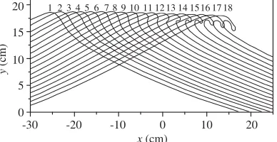
The breaking-wave regions of the sea are derived by the LONGTANK numerical hydrodynamic code that is proposed by Wang et al. at the ocean engineering laboratory of the University of California, Santa Barbara (UCSB) [12]. Figure 1 shows the scattering model of LONGTANK waves, which is consistent with tank experiments and ocean observation.
-30 -20 -10 0 10 20
x (cm) 20
15
10
5
0
y
(cm)
1 2 3 4 5 6 7 8 9 10 11 12 13 14 1516 17 18
Figure 1. The scattering model of LONGTANK breaking waves.
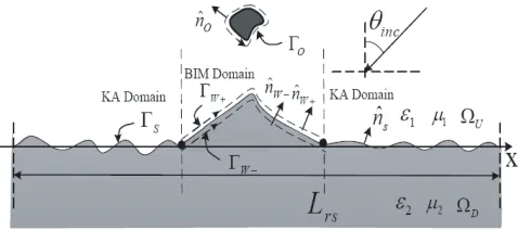
As laboratory profiles of breaking waves are lower than 20 cm, the roughness added on the breaking waves in [8] is associated with a very low wind speed in the Pierson-Moskowitz (PM) spectrum (1.5 m/s). In [8], the roughness is only added to the front face of the breaking wave. In this paper, a simple combined model of the PM roughness added to both the front and back faces of the breaking wave is designed which is more practical. The wave crest is further elongated with straight lines, and the rough sea surface can be generated by the PM spectrum [13]. The parts of the sea surface overlapped by the breaking wave are removed, and the connection points are the crossover points between the PM sea surface and the breaking wave. If the discontinuity appears at the joints between two regions, the discontinuous points near the joint can be removed so that the other points can be connected to obtain continuity and a smoother surface. In our model, the junctions between the PM sea surface and the breaking wave float with the undulation of the sea. Figure 2 gives a two-dimensional (2D) scattering model of a PEC object above the dielectric rough sea surface with the breaking wave. Although the model is not an exact representation of the real sea, it gives a reasonable approximation of the real sea surface for a gentle breeze to some extent.
Figure 2. The 2D scattering model of an object above the sea with breaking wave.
parts, one is the BIM region including the breaking wave and the object, and the other is the KA region including the traditional PM sea surface.
When using a moment-method based approach to numerically model the scattering from the sea surface of unlimited extent, the primary limiting factor is that the sea must be truncated so that the discretized integral equation can be treatable with finite computer resources. To truncate the rough sea to a finite model, a tapered incident wave [14] is chosen as the incident wave, and the form of the incident wave can be expressed as
Φinc(r) = exp [ik·r(1 +w(r))]·exp
−(x−ycotθinc)2/g2
(1)
wherew(r) = [2(x−ycotθinc)2/g2−1]/(kgsinθinc)2,kis a vector of the wavenumber in the space, and ris the position vector. g denotes the tapered factor which is usually adopted a value ofLrs/4.
Firstly, considering the BIM region, total fields in the upper space of the rough sea surface ΩU are governed by the Helmholtz equation for both HH and V V polarizations
∇2Φ(r) +k2
1Φ(r) =f(r) (2)
in which forHHcase, Φ(r) =Ez(r),f(r) =−ik1Z1Jz(r); forV V case, Φ =Hz,f(r) =−[∇×Jz(r)ˆz]·zˆ; Z1 is the characteristic impedance of ΩU;Jz represents the distribution of the current density;k1 is the
wavenumber of ΩU. The following boundary integral equation can be yielded [13]
Φr =
ΓW+
Φ(r)∂G1(r,r
)
∂nW+
dΓ−
ΓW+
G1(r,r) ∂ ∂nW+
Φ(r)dΓ
+γ
ΓO
Φ(r)∂G1(r,r)
∂nO dΓ−(1−γ)
ΓO
G1(r,r) ∂
∂nOΦ(r)dΓ + Φ
incr (3)
where Φinc(r) = −Ω
U[G1(r,r)f(r)]dΩ, G1(r,r) is the Green function [15] in domain ΩU, r is a
position vector in domain ΩU. As the object is a PEC model, the PEC conditions are satisfied on its surface ΓO. For HH polarization, γ = 0; for V V polarization, γ = 1. The scattering field from the object and breaking wave can be calculated by Eq. (3). Expanding the unknowns with the pulse basis functionfn(r) and adopting the point matching algorithm, the following weak form of Eq. (3) can be represented in matrix notation as
[b] = [AW+] [ΦW+] + [BW+] [UW+] +γ[AO] [ΦO] + (1−γ) [BO] [UO] (4)
in which matrices [Φ] and [U] represent Φ and∂Φ/∂n, respectively. The subscriptW denotes the nodes on breaking wave, the subscript O denotes the nodes on the object. The elements of matrices [A], [B], and [b] are defined as follows
AWij+ = firi−
rj+Δl/2
rj−Δl/2
fjrj∂G2(r,r
i) ∂nW+
dl (5)
BijW+ =
rj+Δl/2
rj−Δl/2
fjrj∂G2(r,r
i) ∂nW+
derivations of the integral formulation in the air, one similar field integral equation in the sea water can be obtained as
Φr=−
ΓW−
Φ(r)∂G2(r,r
)
∂nW− dΓ +
ΓW− G2
r,r ∂
∂nW−Φ(r)dΓ (10)
where G2(r,r) denotes the Green’s function in domain ΩD, k2 is the wavenumber in domain ΩD. It
should be noted that the part about the source does not exist, because the incident wave only exists in domain ΩU. Combining Eq. (10) with the pulse basis functionfn(r) and the point matching algorithm, the following matrix equation can be yielded
[AW−] [ΦW−] + [BW−] [UW−] = [0] (11) where
AWij− = firi+
rj+Δl/2
rj−Δl/2
fjrj∂G2(r,r
i)
∂nW− dl (12)
BijW− = −
rj+Δl/2
rj−Δl/2
fjrj∂G2(r,r
i)
∂nw− dl (13)
On the boundary of the breaking wave, the relation between domains ΩU and ΩD can be coupled by boundary continuity conditions which can be written as
Φ|ΓW+ = Φ|ΓW− (14)
1 ρ+ ∂Φ ∂n
ΓW+
= 1 ρ− ∂Φ ∂n
ΓW−
(15)
in which for HH case, ρ = μr; for V V case, ρ = εr. Eqs. (4) and (11) can be contacted with each other by Eqs. (14) and (15). The coupled matrix equations are then solved by the conjugated gradient method (CGM). After the field on the object and breaking wave are worked out, the scattering field on the KA region from BIM region can be obtained by Eq. (3).
Secondly, considering the KA region, the scattering fields and their normal derivations on the boundary ΓS of the PM rough sea can be evaluated by
ΦscatKA (r)Γ
S = R(r) Φ inc(r)
ΓS (16)
∂ΦscatKA (r)
∂n
ΓS
= −R(r)∂Φ
inc(r) ∂n ΓS (17)
So the total field on the rough surface can be expressed as
ΦKA(r)|ΓS = [1 +R(r)] Φinc(r)ΓS (18) ∂ΦKA(r)
∂n
ΓS
= [1−R(r)]∂Φ
inc(r) ∂n ΓS (19)
where the Fresnel reflective coefficients for bothHH case and V V case on the boundary ΓS+ are
R(r) = cosθ− ε2/ε1−sin
2θ
cosθ+ ε2/ε1−sin2θ
For HH case (20)
R(r) = ε2/ε1cosθ− ε2/ε1−sin
2θ ε2/ε1cosθ+ ε2/ε1−sin2θ
whereθ is the local incident angle on the rough surface. Substituting Eqs. (20) and (21) into Eqs. (18) and (19), the field induced by KA region can be yielded by the following boundary integral equation
ΦKA
r=
ΓS
Φ(r)∂G1(r,r
)
∂ns −G1(r,r
) ∂
∂nsΦ(r)
dΓ + Φincr (22)
The scattering field on the BIM region from the KA region can be calculated by Eq. (22).
Now, we consider the interaction between the BIM and KA regions. Before the iteration process begins, the initial fields on both regions are assumed to be zero. Firstly, the field in KA region can be estimated by Eqs. (18) and (19). In the next step, the scattering field on the BIM region from the KA region can be solved by Eq. (22), and the scattering field is added to the incident field in Eq. (3) as a secondary incident wave. Then, the fields on the breaking wave and the target can be worked out by Eqs. (4) and (11). On the basis of the field in BIM region, the scattering field on KA region from BIM region can be calculated by Eq. (3). The iteration goes to the step of solving the field in the KA region by Eqs. (18) and (19), and continues the circulation until the fields in the BIM region reaching convergence, which can be determined by the following equation
ζ =
n
i=1
ΦkBI+1−
n
i=1
ΦkBI
n
i=1
ΦkBI
(23)
where ΦBI is the field in BIM region of each iteration step, ndenotes the total nodes of BIM region, k
is the iteration time. The symbolζ denotes the iterated error, and the iteration can be considered to achieve convergence whenζ <1.0e−4. This process can take the multiple reflections between the BIM region and KA region into account. This hybrid iterative algorithm can be proved to be a powerful electromagnetic simulation tool.
3. PROCEDURE AND CODE VALIDATIONS
Several numerical simulations are considered to demonstrate the general solutions derived here and illustrate the accuracy of our proposed method. In our discussion, the frequency of the incident wave is 1.0 GHz, and the dielectric constant of the sea water is well approximated by ε= 73.82 +i89.26 based on Debye model [16].
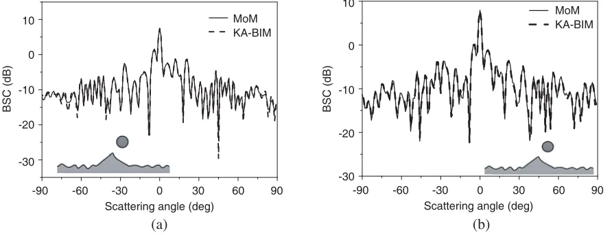
The first example is devoted to simulate the scattering from a PEC circular cylinder above a dielectric rough sea surface, Figures 3(a) and 3(b) give the scattering results of bistatic scattering
-90 -60 -30 0 30 60 90 Scattering angle (deg)
-90 -60 -30 0 30 60 90 Scattering angle (deg)
10
0
-10
-20
-30
BSC (dB)
10
0
-10
-20
-30
BSC (dB)
MoM KA-BIM
MoM KA-BIM
(a) (b)
Figure 3. Scattering from a circular cylinder above the PM sea with breaking wave (profile 6). (a)
new method reduces to 11.13%, and the storage memory in the new method decreases to 1.24%. As a result, the calculation time in KA-BIM decreased greatly in the process of solving the matrix. For HH
case, the filling time of the hybrid method decreases to 2.20% of that in MoM, and the calculation time decreases to 4.93% of that in MoM. For V V case, the filling time is almost same to that of HH case in two methods, but the calculation time is less than that of HH case. The calculation time of new method decreases to 3.62% of that used MoM.
Table 1. Calculation time and number of unknowns in MoM and new method.
Methods Number of
matrix unknowns
Storage
Memory (M)
Filling
time (s)
Calculation
time (s)
Iteration
steps
HH MoM New
method
6790 703.49 94.86 352.56 none
756 8.72 2.09 17.38 2
V V MoM New
method
6790 703.49 98.64 487.59 none
756 8.72 1.92 17.64 2
* Calculated by a computer with a 2.50 GHz processor (Intel (R) Core (TM)2 Quad CPU), 3.47 GB memory.
-90 -60 -30 0 30 60 90
Scattering angle (deg) 10
0
-10
-20
-30
BSC (dB)
MoM KA-BIM
(a) (b)
-90 -60 -30 0 30 60 90
Scattering angle (deg) MoM KA-BIM
-40
10
0
-10
-20
-30
BSC (dB)
-40
-50
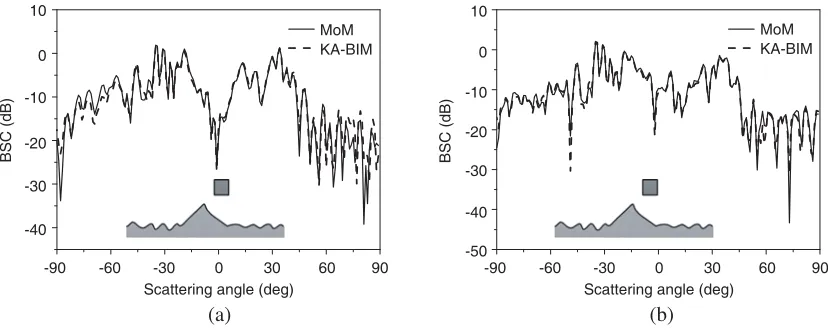
Figure 4. Scattering from a square above the PM sea with breaking wave (profile 18). (a)HH. (b)
V V.
In order to further verify the validation of our algorithm, another numerical example is given in Figures 4(a) and 4(b) for the bistatic scattering from a PEC square above the sea with breaking wave 18. A wind of U19.5 = 2.0 m/s blows the sea with Lrs = 10 m for HH and V V polarizations. The
incident angle is θinc= 30◦. A square with a width of l = 2 m is set ath = 4 m above the sea. It can be seen that both methods are almost perfectly matched for bothHH and V V polarizations.
Table 2. Calculation time and number of unknowns in MoM and new method.
Methods Number of
matrix unknowns
Storage
Memory (M)
Filling
time (s)
Calculation
time (s)
Iteration
steps
HH MoM New
method
6950 737.04 106.83 390.19 none
940 13.48 2.13 43.15 2
V V MoM New
method
6950 737.04 104.39 528.12 none
940 13.48 2.44 46.28 3
* Calculated by a computer with a 2.50 GHz processor (Intel (R) Core (TM)2 Quad CPU), 3.47 GB memory.
Figure 5. Scattering model of a NACA2412 airfoil above the sea with breaking waves.
0 10 20 30 40 50 60
Incident angle (deg)
(a) (b)
10
0
-5
-10
-15
MSC (dB)
-20
-25 5
10
0
-5
-10
-15
MSC (dB)
-20
-25 5
70 80 0 10 20 30 40 50 60
Incident angle (deg)
70 80 wave1
wave6 wave12 wave18
wave1 wave6 wave12 wave18
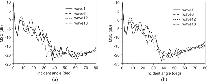
Figure 6. Scattering for an airfoil above the sea with different breaking waves. (a)HH. (b)V V.
the storage memory in KA-BIM is reduced to 1.83% of that in MoM. It can be seen from Table 2 that KA-BIM consumes very little simulation time compared with that of MoM. The filling time in the new method decreases to about 1.99% and 2.34% of that in MoM for HH and V V cases. Compared with MoM, the calculation time of the new method is reduced to 11.06% for HH case and 8.76% for V V
case.
0 10 20 30 40 50 60 Incident angle (deg)
(a) (b)
70 80 0 10 20 30 40 50 60 Incident angle (deg)
70 80
-30 -30
Figure 7. Scattering for an airfoil above the sea with breaking wave 6 for different wind speeds. (a)
HH. (b)V V.
average their scattering field to obtain a stable result.
The influence on monostatic scattering coefficient (MSC) with the evolution of the breaking waves is studied. Figure 6 shows the scattering coefficients for HH and V V cases when the breaking wave develops from profile 1 to profile 18. For bothHH andV V cases, the scattering shows an increase near 10◦ as the breaking wave develops.
The scattering results of the model of breaking wave 6 on the sea for HH and V V polarizations are given in Figures 7(a) and 7(b). The scattering coefficient near 10◦ increases with the wind speed increasing. In our model, it also can be seen from Figure 7 that the scattering coefficient for HH have a more clear variation thanV V case in some angles. From 35◦ to 65◦, the MSC shows an increase when the wind speed varies from 1.0 m/s to 2.0 m/s. On the contrary, the scattering coefficient decreases from 70◦ to 80◦.
4. CONCLUSIONS
In this paper, an iterative analytical-numerical method is designed to study two-dimensional electromagnetic scattering from a target located above the sea with breaking waves. Based on the geometrical model of a target above the sea with breaking waves, an iterative KA-BIM is developed to study the approximate model of the realistic sea for the first time. In the iterative algorithm, the initial fields on the traditional PM sea surface can be estimated by KA. Then the scattering field deduced by KA region on the BIM region can be obtained. The scattering wave from the KA region can be seen as an incident source which impinges upon the target and the breaking wave. Based on the BIM theory, the field information on the target and the breaking wave can be worked out. After iteration, the scattering model is able to yield stable and precise results when the fields on the target and the breaking wave reach convergence. To improve the simulation precision of the scattering from the sea, the whole sea is divided into two regions: breaking wave region and PM sea region. The scattering from the breaking waves is exactly studied by BIM, and KA is used to analyze the scattering from the PM sea. The numerical comparisons show that the hybrid method can not only provides accurate results but also save lots of memory and calculation time. It is worthwhile to note that by combining the hybrid method with accelerated boundary integral method, such as FBM and MLFMA, the efficiency of the hybrid method can be further improved.
ACKNOWLEDGMENT
REFERENCES
1. Holliday, D., L. L. De Raad, Jr., and G. J. St-Cyr, “Sea-spike backscatter from a steepening wave,”
IEEE Trans. Antennas Propagat., Vol. 46, 108–113, 1998.
2. West, J. C., “Low-grazing-angle (LGA) sea-spike backscattering from plunging breaker crests,”
IEEE Trans. Geosci. Remote Sens., Vol. 40, 523–526, 2002.
3. Zhao, Z. and J. C. West, “Low-grazing-angle microwave scattering from a three-dimensional spilling breaker crest: A numerical investigation,” IEEE Trans. Geosci. Remote Sens., Vol. 43, 286–294, Feb. 2005.
4. Li, Y. and J. C. West, “Low-grazing-angle scattering from 3-D breaking water wave crests,” IEEE
Trans. Geosci. Remote Sens., Vol. 44, 2093–2101, 2006.
5. Qi, C., Z. Zhao, W. Yang, Z.-P. Nie, and G. Chen, “Electromagnetic scattering and Doppler analysis of three-dimensional breaking wave crests at low-grazing angles,” Progress In Electromagnetics
Research, Vol. 119, 239–252, 2011.
6. Yang, W., Z. Zhao, C. Qi, and Z. Nie, “Electromagnetic modeling of breaking waves at low grazing angles with adaptive higher order hierarchical legendre basis functions,” IEEE Trans. Geosci.
Remote Sens., Vol. 49, 346–352, 2011.
7. Luo, W., M. Zhang, C. Wang, and H.-C. Yin, “Investigation of low-grazing-angle microwave backscattering from three-dimensional breaking sea waves,”Progress In Electromagnetics Research, Vol. 119, 279–298, 2011.
8. West, J. C. and Z. Q. Zhao, “Electromagnetic modeling of multipath scattering from breaking water waves with rough faces,”IEEE Trans. Geosci. Remote Sens., Vol. 40, 583–592, 2002. 9. Ye, H. and Y. Q. Jin, “Fast iterative approach to difference scattering from the target above a
rough surface,”IEEE Trans. Geosci. Remote Sens., Vol. 40, 108–115, 2006.
10. Kubicke, G., C. Bourlier, and J. Saillard, “Scattering from canonical objects above a sea-like one-dimensional rough surface from a rigorous fast method,” Waves in Random and Complex Media, Vol. 20, 156–178, Jan. 2010.
11. Ye, H. and Y.-Q. Jin, “A hybrid analytic-numerical algorithm of scattering from an object above a rough surface,” IEEE Trans. Geosci. Remote Sens., Vol. 45, 1174–1179, 2007.
12. Wang, P., Y. Yao, and M. P. Tulin, “An efficient numerical tank for nonlinear water waves, based on the multi-subdomain approach with BEM,”Int. J. Numer. Methods Fluids, Vol. 20, 1315–1336, 1995.
13. Tsang, L., J. A. Kong, K. H. Ding, and C. O. Ao,Scattering of Electromagnetic Waves: Numerical
Simulations, Wiley, New York, 2001.
14. Thorsos, E. I., “The validity of the Kirchhoff approximation for rough surface scattering using a Gaussian roughness spectrum,”J. Acous. Soc. Am., Vol. 83, 78–92, 1988.