Radar Target Recognition by Frequency-Diversity RCS Together with Kernel Scatter Difference Discrimination

(1)

Radar Target Recognition by Frequency-Diversity RCS Together

with Kernel Scatter Diﬀerence Discrimination

Kun-Chou Lee*

Abstract—In this paper, the radar target recognition is given by frequency-diversity RCS (radar cross section) together with kernel scatter difference discrimination. The frequency-diversity technique means to collect electromagnetic signals by sweeping the operation frequencies. Such a technique is usually utilized in inverse scattering and radar target recognition because different frequencies each may contain important information of a target. By using the frequency diversity RCS technique, one can reduce the times of spatial measurement. This is an important contribution since it is always difficult to build a spatial radar measurement in practical battlefield environments. To enhance pattern recognition, the collected RCS data are processed by the kernel scatter difference discrimination, which is improved from the Fisher discrimination. To investigate the capability of tolerating environmental fluctuation, each simulated RCS data is added by a random component prior to implementing pattern recognition. Numerical simulation shows that our recognition scheme is still very accurate even though the RCS contains a random component.

1. INTRODUCTION

The efficiency of a weapon system directly depends on the target recognition capability of a radar system in modern battlefield environments [1]. Traditional radar identification technology usually utilizes a target’s images for identification, e.g., SAR (synthetic aperture radar) [2, 3] and ISAR (inverse synthetic aperture radar) [4, 5]. Although these techniques work well, radar images are difficult to obtain due to the expensive hardware. In general, measuring RCS (radar cross section) [6, 7] is easier than achieving radar images. This motivates us to implement target recognition through RCS. The RCS is affected by frequencies, spatial directions and polarizations. Target recognition by original RCS usually involves enormous data computations. To achieve efficient and reliable recognition, the original RCS data are often projected to an eigenspace prior to identification. The goal is to reduce the data complexity and enhance the discrimination.

Practically, the techniques of collecting electromagnetic signals for inverse scattering are divided into three categories, which are angular, frequency and polarization diversities [8, 9]. Among these three techniques, the frequency diversity [10, 11] is the most efficient so that it becomes very important in inverse scattering. Such a diversity technique means to collect electromagnetic signals by sweeping the operation frequencies. In general, a target always contains special information at different frequencies. Physically, the radar target recognition is a simple and rough approach of inverse scattering. Therefore, it is reasonable to expect that the frequency diversity technique is also useful in RCS based target recognition. Compared with angular-diversity RCS (i.e., collecting electromagnetic signals by changing spatial angles) [12–14], the frequency-diversity RCS technique is more efficient and contains much more

Received 12 October 2019, Accepted 2 December 2019, Scheduled 16 December 2019 * Corresponding author: Kun-Chou Lee ([email protected]).

(2)

information for identiﬁcation. This then motivates us to implement radar target recognition by using frequency-diversity RCS.

In this paper, the radar target recognition is given by frequency-diversity RCS together with kernel scatter difference discrimination [14–16]. The kernel scatter difference discrimination [14–16] improves conventional Fisher discrimination [17] in computational efficiency, but is not affected by the matrix singularity. Such a pattern recognition technique is based on the differences between “kernel between-class” and “kernel within-class” matrices of scatters. The “kernel between-class” scatter matrix represents the mean distance between centers of different classes in eigenspace, and is expected to be as large as possible. Whereas the “kernel within-class” scatter matrix represents the mean distance between samples within the same class and their center, and is expected to be as small as possible. Thus one can calculate the eigenvalues and eigenvectors in eigenspace. Initially, the frequency-diversity RCS data are collected and projected to the eigenspace. Next, eigenvectors corresponding to several largest eigenvalues are selected as the principal components in eigenspace. Finally, the Euclidean distance in eigenspace is calculated for identifying types of targets. Numerical simulation shows that our radar target recognition scheme can identify targets accurately and efficiently, even though there exist random noises.

In the following, theoretical formulations are given in Section 2. Numerical simulation results are given in Section 3. Finally, conclusions are given in Section 4.

2. FORMULATIONS

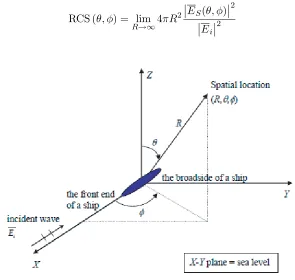
This study has no limitation on the types of targets. With loss of generality, we utilize the ship model as the target for simplicity. Consider a ship on the sea level (X-Y plane), as shown in Fig. 1. The front end and broadside of a ship are in directions of +X and ±Y, respectively. A spatial location is characterized by spherical coordinates (R,θ,φ), whereR is the distance to the coordinate origin,θ the elevation angle, and φthe azimuth angle. The ship is illuminated by a horizontally propagating plane wave Ei with ˆz-polarization and unit magnitude. This incident wave will produce a scattered electric

field and then the RCS. The RCS means the relative power magnitude of the reflected electromagnetic signals from a target. Mathematically, the bistatic RCS in the direction of (θ,φ) is defined as [6]

RCS (θ, φ) = lim

R→∞4πR

2ES(θ, φ) 2

_E_i2 (1)

(3)

whereEi is the incident electric ﬁeld, andES(θ, φ) is the scattered electric ﬁeld. As mentioned above,

a target always contains special information at diﬀerent frequencies. Therefore, this study utilizes frequency-diversity technique to collect RCS data for target identiﬁcation.

Our recognition scheme includes two stages, which are training and testing. In the training stage, we ﬁrst select training vectors. Assume there are P (p= 1, ..., P) categories of known ships. For each ship in Fig. 1, the incident wave horizontally propagates toward the target from the azimuth angles of φi = 0◦, 90◦ and 180◦, sequentially. For each incident azimuth angle (φi), the RCS data are collected

in the direction of (θ,φi) whereθis changed asθ1,θ2, ..., andθN, sequentially. For each direction, the

operation frequency is swept as f1, f2, ..., and fM, sequentially. Thus we have a frequency-diversity

signal matrix with the dimension of (3M)×(N P), as shown in Fig. 2.

category #1 category #2 category #3

fishing boat naval ship container vessel

RCS RCS RCS RCS RCS RCS RCS RCS RCS

. . . . . . . . . . . . . . . . . . . . . . . . . . . . . . . . . . . . . . . . . . . . . . . . . . . . . . . . . . . . . . . . . . . . . . . . . . . . . . . . . . . . . . . . . . . . . . . . . . . . . . . . . . . . . . . . . . . . . . . . . . . . . . . . . . . . . . .

φ = 0

φ = 90

φ = 180 i i i o o o f f f 1 2 M f f f 1 2 M f f f 1 2 M

θ1 θ2 θN θ1 θ2 θN θ1 θ2 θN

Figure 2. Illustration of the frequency-diversity signal matrix.

This study utilizes the kernel scatter difference discrimination [14–16] for identification. The details of kernel scatter difference discrimination can be found in References [14–16]. The pattern recognition procedures are briefly given in the following. Assumexp_i denotes thei-th column in category #pof Fig. 2. It is a training vector in the original RCS data space. In the kernel scatter difference discrimination [14– 16], xp_i is projected to a higher dimensional feature spaceF through a mapping function Φ(·) as

xp_i →Φ(xp_i)∈F, p= 1,2, ..., P; i= 1,2, ..., N. (2)

In the kernel mapping, the “kernel between-class” scatter matrixKB and “kernel within-class” scatter

matrixKW are deﬁned as [14–16]

KB =

P

p=1

(4)

and

KW =

1 N P p=1 N i=1

δp_i −up

·δp_i −up

_T

(4)

where

up =

1 N

_N

i=1

κx11, xp_i

, ...,

N

i=1

κ(x1_N, xp_i), ... ...,

N

i=1

κ(xP1, xp_i), ..., N

i=1

κ(xP_N, xp_i)

T

(5)

δp_i = κ(x11, xp_i), ..., κ(x1N, xpi), ... ..., κ(xP1, xp_i), ..., κ(xPN, xpi)

T

(6)

and

umean=

1

N·P

P p=1 N i=1

δp_i. (7)

The symbol “T” in Eqs. (3)–(6) denotes the transposition. The notationκ(·) in Eqs. (5)–(6) is a kernel transformation, which is deﬁned as

κ(x, y) = (x·y)d (8)

wheredis the kernel polynomial degree [14–16]. The scatter-diﬀerence based discrimination function is given as [14–16]

J(ε) =εT

KB−·KW

ε (9)

whereεis the optimal transformation matrix, andis the impact parameter. By adjusting the impact parameter in Eq. (9), one can control the impact from KB or KW. The optimal transformation

matrix in Eq. (9) is given as ε = (ω1, ω2, ..., ωe) where ω1, ω2, ..., and ωe are principal eigenvectors.

These principal eigenvectors will be introduced later. As all training vectors are mapped via the optimal transformation matrixε, the discrimination function J(ωi) in Eq. (9) will be maximized. That is, the

“kernel between-class” scatter matrix KB is maximized and the “kernel within-class” scatter matrix

KW is minimized. This is the optimal discrimination and then the goal of pattern recognition.

Each principal eigenvector is normalized as ω_i = 1, i = 1,2, ..., e. Thus maximizing J(ωi) is

equivalent to ﬁnding the maximum of the Lagrange function L(ωi, λ) [14–16] where

L(ωi, λ) =J(ωi)−λ(ωi −1), i= 1,2, ..., e. (10)

By taking the partial diﬀerential of the above function with respect toωi and setting the result to be

zero, we have

KB−·KW

ωi =λωi. (11)

There are NP eigenvalues (i.e., solutions of λ) in Eq. (11) and these eigenvalues are ranked as λ1 ≥ λ2 ≥ ... ≥ λN P. We select the top e (e < N P) eigenvalues (λ1 ≥ λ2 ≥ ... ≥ λe) and their

corresponding eigenvectors ω1, ω2, ..., ωe as principal components for eigenspace of kernel scatter

diﬀerence. That is, principal eigenvectors ω1, ω2, ..., ωe will span the eigenspace of kernel scatter

diﬀerence.

After constructing the eigenspace through the principal eigenvectors, one can project an arbitrary signal vector x to a higher dimensional space and then to the eigenspace. The resulting feature vector is

Ω = (ω1, ω2, ..., ωe)T ·

κ(x11, x), ..., κ

x1_N, x, ... ..., κxP1, x

, ..., κxP_N, x. (12)

All training vectors are projected to the eigenspace by Eq. (12). The center or mean of feature vectors for each category in eigenspace is calculated as

Ω_meanp = 1 N

N·p

i=1+N(p−1)

(5)

In the testing stage, the RCS vector x of an unknown target is collected, mapped to the feature space F, and then projected to the eigenspace by Eq. (12). Thus, an e-dimensional feature vector Ω as Eq. (12) is obtained. Finally, the Euclidean distance from the testing vector to the center of each category in eigenspace is calculated as

Γ_p =Ω−Ω_meanp , p= 1,2, ..., P. (14)

One can use the Euclidean distance of Eq. (14) to estimate the similarity between the unknown and known targets. If the testing vector is the closest (i.e., with the smallest Euclidean distance) to thep-th category, we judge the unknown target to be a ship of thep-th category.

3. NUMERICAL SIMULATION RESULTS

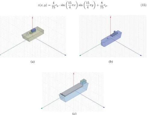
In this section, numerical examples are given to verify the above formulations. For simplicity, models of ships are considered as targets instead of real ships. As illustrated in Fig. 3, there are three categories of ships (P = 3) for modeling the ﬁshing boat (category #1), naval ship (category #2) and container vessel (category #3). The ship size is kr1 = 3.1 for category #1, kr2 = 6.3 for category #2, and kr3 = 9.4

for category #3, where k is the wavenumber, and rp (p = 1, 2, 3) represents the length of a ship. All

ships are assumed to be on the sea level (X-Y plane) and the characteristic for surface roughness of sea water is assumed to be

z(x, y) = 4

75rp·sin

15 4 πx

sin

15 4 πy

+ 8

75rp. (15)

(a) (b)

(c)

(6)

The sea water has a dielectric constant εr = 81 and conductivity σ= 4 S/m. In numerical simulation,

we utilize the Ansys HFSS (High Frequency Structure Simulator) software to calculate the RCS of ships. In the training stage, the frequency-diversity signal matrix is ﬁrst constructed. For each incident azimuth angle (φi = 0◦ or 90◦ or 180◦), the RCS data are collected in the direction of (θ, φi) where

θ is changed as θ1 = 61◦, θ2 = 63◦, ..., and θ15 = 89◦, sequentially. For each direction, the operation

frequency is swept as f1 = 3.1 GHz, f2 = 3.2 GHz, ..., and f10= 3.9 GHz. Thus we have a

frequency-diversity signal matrix with the dimension of 30×45, as shown in Fig. 2.

In the testing stage, the arrangement for collecting the RCS of an unknown ship is the same as that of the training stage, except that the evaluation angles are changed as θ1 = 62◦, θ2 = 64◦, ...,

and θ15 = 90◦. Note that the evaluation angles of the testing stage are diﬀerent from those of the

training stage. Such an arrangement is for investigating the ability to identify examples that have not been learned. Our goal is to identify which training (known) ship is the most similar to the testing (unknown) ship by using Eq. (14). In our treatment, the number of principal components (e) and the kernel polynomial degree (d) are set to bee=d= 1 based on research experiences.

In the ﬁrst example, we choose the ship of category #1 (i.e., a ﬁshing boat) as the tested (unknown) target. Following the procedures of Section 2, the distance to feature’s center of each category is calculated by Eq. (14) and then given in Fig. 4. From Fig. 4, it is shown that the line of Γ1is the lowest

for each testing elevation angleθ. Thus we judge the unknown target to be a ﬁshing boat (i.e., category #1 of known ships). This recognition result is consistent with the fact. The judgments are all correct for all the 15 testing elevation angles. The correct recognition rate is 100% (15/15).

60 70 80 90

distance

tested target: category #1

Γ (distance to features' center of category #1)

Γ (distance to feature's center of category #2)

testing elevation angle θ (deg) 50000

40000

30000

20000

10000

0

1 2 3

Figure 4. The distance to feature’s center of each category by using the ship of category #1 (i.e., a ﬁshing boat) as the tested target.

60 70 80 90

distance

30000

20000

10000

0

1 2 3

Figure 5. The distance to feature’s center of each category by using the ship of category #2 (i.e., a naval ship) as the tested target.

In the second example, we choose the ship of category #2 (i.e., a naval ship) as the tested (unknown) target. The other arrangements are the same as those of the ﬁrst example. The distance to feature’s center of each category is calculated by Eq. (14) and then given in Fig. 5. Fig. 5 shows that the line of Γ2 is the lowest for each testing elevation angle θ. Thus we judge the unknown target to be a naval ship

(i.e., category #2 of known ships). This recognition result is consistent with the fact. The judgments are all correct for all the 15 testing elevation angles. The correct recognition rate is 100% (15/15).

(7)

60 70 80 90

distance

40000

30000

20000

10000

0

1 2 3

Figure 6. The distance to feature’s center of each category by using the ship of category #3 (i.e., a container vessel) as the tested target.

0.0001 0.001 0.01 0.1 1

normalized standard deviation of noise 95

96 97 98 99 100

successful recognition rate (%)

100 100 100 100

99.44

95.8

Figure 7. The successful recognition rate with respect to diﬀerent levels of random noises.

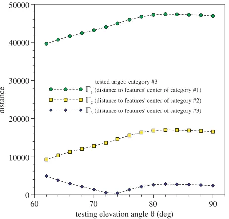
that the line of Γ3 is the lowest for each testing elevation angleθ. Thus we judge the unknown target

to be a container vessel (i.e., category #3 of known ships). The recognition result is consistent with the fact. The judgments are all correct for all the 15 testing elevation angles. The correct recognition rate is 100% (15/15). From the above three examples, the overall successful recognition rate is 100% (45/45).

To understand whether the proposed recognition scheme is aﬀected by noises, we add a random component to each computed RCS. The random component is generated by Gaussian distribution with zero-mean. The standard deviation of noise distribution is normalized by the root-mean-square RCS and is chosen as 10−4, 10−3, 10−2, 10−1, 2×10−1, and 4×10−1, respectively. Fig. 7 shows the successful recognition rate with respect to diﬀerent levels of random noises for our recognition scheme. The noise level here means the normalized standard deviation of random components. From Fig. 7, it shows that the successful recognition rate is 100%, 100%, 100%, 100%, 99.44%, and 95.8%, for noise levels of 10−4, 10−3, 10−2, 10−1, 2×10−1, and 4×10−1, respectively. Fig. 7 reports that the successful recognition rate is still greater than 95%, even though the noise level is increased to 4×10−1. This implies that the proposed recognition scheme has very good ability to tolerate random noises.

Figure 8 shows the successful recognition rate with respect to the number of principal components (e) under diﬀerent choices of kernel polynomial degree (d). In Fig. 8, the noise level is set as 4×10−1_,

i.e., the worst case of noise effects. Fig. 8 reports that the recognition rate is always greater than 90% for all choices of principal components (e) and kernel polynomial degree (d). This implies that the kernel scatter difference discrimination is a very good pattern recognition technique in such a problem. Fig. 8 also reports that the kernel polynomial degree (d) is an important factor in our recognition scheme, whereas the impact from the number of principal components (e) is not significant.

In Eq. (9), the scatter-diﬀerence based discrimination function is aﬀected by the kernel between-class scatter matrixKBand kernel within-class scatter matrixKW. The weight of impact fromKBand

KW are controlled by adjusting the impact parameter (). Fig. 9 shows the successful recognition rate

(8)

15 20 25 30 35 40 45 number of principal components (e)

88 89 90 91 92 93 94 95 96 97

polynomial degree d = 1

0 5 10

polynomial degree d = 2 polynomial degree d = 3 polynomial degree d = 4

Figure 8. The successful recognition rate with respect to the number of principal components (e) under diﬀerent choices of kernel polynomial degree (d).

50 60 70 80 90 100

60 70 80 90 100 50

0 10 20 30 40

values of impact parameter ( )

Figure 9. The successful recognition rate with respect to diﬀerent values of impact parameter ().

4. CONCLUSIONS

In this paper, the radar target recognition is successfully implemented by frequency-diversity RCS together with kernel scatter difference discrimination. The frequency-diversity RCS technique of this study required 3× 15 = 45 spatial directions (i.e., 3 azimuth angles and 15 elevation angles) in constructing the signal matrix for target recognition. Whereas the target recognition by angular-diversity RCS techniques [12–14] requires 181×15 = 2715 spatial directions (i.e., 181 azimuth angles and 15 elevation angles) in constructing the signal matrix for target recognition. Note that it is always difficult to build a spatial radar measurement in practical battlefield environments. The frequency diversity RCS technique of this study has indeed reduced the times of spatial radar measurement and is then an important contribution in target recognition. To enhance the discrimination, this study utilizes kernel scatter difference technique of pattern recognition. Numerical simulation shows that our target recognition scheme not only gives accurate identification but also significantly reduces the data dimension. The target recognition scheme in this study can also be applied to many other problems of radar engineering.

ACKNOWLEDGMENT

The authors would like to thank (1) the ﬁnancial support from the Ministry of Science and Technology, Taiwan, under Grant MOST 108-2221-E-006-091, (2) the National Center for High Performance Computing, Taiwan, for computer time and facilities, and (3) Dr. Sheng-Chih Chan for his help in this study.

REFERENCES

(9)

2. Osman, H., L. Pan, S. Blostein, and L. Gagnon, “Classiﬁcation of ships in airborne SAR imagery using backpropagation neural networks,” Proceedings of the SPIE Radar Processing, Technology,

and Applications II, Vol. 3161, 126–136, San Diego, USA, September 24, 1997.

3. Zhou, J., Z. Shi, X. Cheng, and Q. Fu, “Automatic target recognition of SAR images based on global scattering center model,” IEEE Transactions on Geoscience and Remote Sensing, Vol. 49, 3713–3729, 2011.

4. Martorella, M., E. Giusti, L. Demi, Z. Zhou, A. Cacciamano, F. Berizzi, and B. Bates, “Target recognition by means of polarimetric ISAR images,” IEEE Transactions on Aerospace and Electronic Systems, Vol. 47, 225–239, 2011.

5. Musman, S., D. Kerr, and C. Bachmann, “Automatic recognition of ISAR ship image,” IEEE

Transactions on Aerospace and Electronic Systems, Vol. 32, 1392–1403, 1996.

6. Ruck, G. T., D. E. Barrick, W. D. Stuart, and C. K. Krichbaum, Radar Cross Section Handbook, Vol. 1, Plenum, New York, 1970.

7. Lee, S.-J., I.-S. Choi, B. Cho, E. J. Rothwell, and A. K. Temme, “Performance enhancement of target recognition using feature vector fusion of monostatic and bistatic radar,” Progress In Electromagnetics Research, Vol. 144, 291–302, 2014.

8. Lee, K. C., “Polarization eﬀects on bistatic microwave imaging of perfectly conducting cylinders,” Master Thesis, National Taiwan University, Taipei, Taiwan, 1991.

9. Farhat, N. H., “Microwave diversity imaging and automated target identiﬁcation based on models of neural networks,” Proceedings of the IEEE, Vol. 77, 670–681, 1989.

10. Chi, C. and N. H. Farhat, “Frequency swept tomographic imaging of three-dimensional perfectly conducting objects,”IEEE Transactions on Antennas and Propagation, Vol. 29, 312–319, 1981. 11. Farhat, N. H., T. Dzekov, and E. Ledet, “Computer simulation of frequency swept imaging,”

Proceedings of the IEEE, Vol. 64, 1453–1454, 1976.

12. Chan, S. C. and K. C. Lee, “Radar target identiﬁcation of ships by kernel principal component analysis on RCS,”Journal of Electromagnetic Waves and Applications, Vol. 26, 64–74, 2012. 13. Chan, S. C. and K. C. Lee, “Radar target recognition by MSD algorithms on angular diversity

RCS,” IEEE Antennas and Wireless Propagation Letters, Vol. 12, 937–940, 2013.

14. Chan, S. C. and K. C. Lee, “Angular-diversity target recognition by kernel scatter-diﬀerence based discriminant analysis on RCS,”International Journal of Applied Electromagnetics and Mechanics, Vol. 42, 409–420, 2013.

15. Liu, Q. S., X. Tang, H. Q. Lu, and S. D. Ma, “Kernel scatter-diﬀerence based discriminant analysisfor face recognition,” Proceedings of the International Conference on Pattern Recognition, Vol. 2, 419–422, Cambridge, UK, August 26, 2004.

16. Liu, Q. S., X. Tang, H. Q. Lu, and S. D. Ma, “Face recognition using kernel scatter-diﬀerence based discriminant analysis,”IEEE Transactions on Neural Networks, Vol. 17, 1081–1085, 2006.