A Real-Time Automatic Method for Target Locating under
Unknown Wall Characteristics in Through-Wall Imaging
Hua-Mei Zhang*, Sheng Zhou, Cheng Xu, and Ye-Rong Zhang
Abstract—To solve the real-time through-wall detection problem in the presence of wall ambiguities, an approach based on kernel extreme learning machine (KELM) is proposed in this paper. The wall ambiguity and propagation effect are included in single-hidden-layer feedforward networks, and then the technique converts the through-wall problem into a regression problem. The relationship between the scattered data and the target properties is determined after the KELM training process. Numerical results demonstrate the good performance in terms of the effectiveness, generalization, and robustness. Compared with the support vector machine (SVM) and least-squares support vector machine (LS-SVM), the KELM provides almost the same estimated accuracy but at a much faster learning speed, which greatly contributes to solving the real-time detection problem. In addition, the situations of two targets, different target radii, and noisy circumstances are discussed.
1. INTRODUCTION
Great interest exists in sensing through obstacles such as brick, wood, concrete blocks, and other visually opaque materials using remote sensing tools whether in civilian applications or military affairs. Through-wall radar imaging (TWRI) is nondestructive technique for detecting and imaging targets behind walls of unknown composition using microwave signals.
Different from the case in free space, the propagation phenomenology in layered media makes the TWRI problem more difficult and challenging. To obtain accurate locations and high quality focused images, compensation for the wall effects must be taken into account in locating and imaging procedures. Thus, wall parameters such as the permittivity, wall thickness, and conductivity play a critical role in TWRI. Ambiguities in the wall parameters will shift the imaged targets away from their true positions, and smear and blur the image. However, in practical situations, the wall parameters are unknown in most circumstances.
However, several techniques have been proposed to provide excellent performance without knowledge of the wall parameters. One kind of method is based on wall parameter estimation. The time-delay approach estimates the wall parameters through the time time-delay produced by different intervals between antennas [1]. Consequently, two measurements are needed, which is time-consuming. Through constructing the cost function between the wall parameters and a computer index, such as the sharpness of the target images and the entropy [2, 3], the cost functional methods attempt to minimize the cost function to obtain the wall parameters. The approximate procedures generally suffer from false solutions and are computationally demanding. To obtain a quick and precise estimation of wall parameters, filter-based methods according to the equivalent propagation model are proposed [4]. The filters are constructed to remove the wall effects in the echo domain or in the image domain, then the estimation
Received 11 November 2019, Accepted 8 February 2020, Scheduled 17 February 2020
* Corresponding author: Hua-Mei Zhang ([email protected]).
methods are converted to obtain the optimization parameters of the filters on the basis of the best focusing quality.
Another method is to directly locate the targets or image through unknown walls. Linear inverse scattering algorithms based on the first-order Born approximation [5], the autofocusing approach based on the spectrum Green’s function [6], etc. all automatically include the effect of walls in the imaging formulation through the multilayer Green’s function and are thus successful in determining the locations and geometrical features of the targets. However, these algorithms have relative difficulty in obtaining a closed-form solution from Sommerfeld integrals. In addition, the trajectory intersection method has been proposed [7, 8]. By setting two different structures of the array or different stand-off distances from the wall, the assumed parameters generate two different displacement trajectories, the intersections of which are the true positions of the targets. These methods have high accuracy and a satisfactory imaging quality, but require at least two measurements, which is time-consuming.
Actually, all the above approaches for TWRI under ambiguous wall parameters aim to find the relationship between the received signals that we can obtain directly and the target properties that we want to know, such as the location, shape, and electromagnetic parameters. In the presence of a wall, the relationship is nonlinear, ill-posed, and difficult to determine. A new approach based on machine learning, such as support vector machine (SVM) and least-squares support vector machine (LS-SVM), is used for this regression problem and able to determine the relationship [9]. The primary problems are converted into quadratic programming (QP) problems, which are solved via the optimization method. Although the SVM achieves a good performance, such as well-defined generalization properties and ability to obtain the global optimal solution, the QP problems are usually tedious and time-consuming [10]. The LS-SVM is one of the main variants of the SVM and uses equality constraints instead of the inequality constraints adopted in the conventional SVM. The LS-SVM avoids QP problem and has smaller computational complexity than SVM. However, the computational time still does not satisfy the request for real-time functionality.
To increase the learning speed, an emergent neural network technology called the extreme learning machine (ELM) has recently become increasingly attractive. The ELM was proposed by Huang et al. in 2004 and originally inspired by biological learning [11]. ELMs were originally developed for single-hidden-layer feedforward neural networks and then extended to “generalized” single-hidden-layer feedforward networks (SLFNs), which may not be neural [12]. From the point of view of network architecture, the SVM and LS-SVM can also be considered as a specific type of SLFN [13]. The ELM learning approach can be applied to SVMs directly by simply replacing the SVM kernels with (random) ELM kernels [13]; thus, it can be used in regression applications such as TWRI. The crucial problem of SLFNs is to determine the hidden layer (also called feature mapping), including the hidden nodes. The standard ELM network has n input neurons, L random hidden nodes, the activation function, and m
output neurons. However, it is a learning process based on the principle of empirical risk minimization, and overfitting cannot be avoided. The generalization and robustness of the standard ELM are affected. Then the orthogonal projection method can be efficiently introduced into the ELM. The generalization and robustness are improved, but the learning efficiency is reduced in optimizing the regularization parameters. A kernel is introduced, which is unknown and used as in the SVM. In the kernel ELM (KELM) algorithm, a kernel matrix consists of a hidden layer feature mapping that does not need to be known to users and can be determined according to the Mercer condition. The Mercer condition means that every semipositive definite function can be a kernel function. The number of hidden nodesL(the dimensionality of the hidden layer feature space) also need not be specified [14]. Thus, compared to traditional ELM algorithms, the KELM using kernel mapping instead of random mapping can effectively improve the generalizability and stability. In addition, better than the SVM and LS-SVM, the hidden layer feature mapping in the KELM can also be known to users [15]. A parameter-insensitive kernel with an analytic form can then be obtained for the ELM for regression, which significantly reduces the computational complexity [13]. The computational efficiency and reliability make the ELM algorithm suitable for real-time applications, especially in TWRI.
used in this paper. In the KELM algorithm, the received signals are considered as the input neurons, and the target location is considered as the output neuron. Thus, the nonlinear relationship is determined by the kernel matrix of the KELM algorithm. This means that through the KELM training process, the model of the nonlinear relationship will be obtained by using the training data. Then, according to the model, the test data will be estimated by using the testing process. To the best of our knowledge, an ELM for real-time automatic detection has not been addressed in prior works in the context of TWRI. The remainder of this paper is organized as follows. Section 2 presents the imaging geometry of the location problem. In Section 3 the theory of the ELM is briefly reviewed, and then the ELM approach for addressing TWRI in the presence of wall parameter uncertainties is presented. Section 4 provides some numerical examples, and the paper concludes in Section 5.
2. MATERIALS AND METHODS
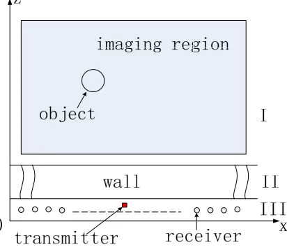
A schematic of the through-wall geometry is shown in Fig. 1. The investigation domain is D = [0,2.4]×[0.4,3] m2. The thickness, conductivity, and relative permittivity of the wall are d = 0.1 m,
εr= 4.5,σ = 0.01 S/m, respectively. A circular cylinder metal target is situated behind the wall. The
radius ρc is 5 cm. A bistatic synthetic aperture radar (SAR) system is used in this paper. A UWB
impulse radar system with one Hertzian dipole placed at the center of the wall along the x-direction transmits a UWB short pulse, namely, a 1.2-ns Gaussian pulse modulated by a 2-GHz cosine wave. The 3-dB frequency bandwidth (BW) is 1.09 GHz, and the start and end frequencies are 1.47 GHz and 2.56 GHz, respectively. Meanwhile, one receiving antenna moves along the x-direction and receives the electric field at N sampling points with equal intervals of 0.02 m. Then, an N-element aperture is synthesized. The number of sampling points is N = 119, and the measurement aperture is 2.4 m.
Figure 1. Schematic of the through-wall geometry.
The simulations are performed using the finite-difference time-domain (FDTD) method, which is an exact field computation method that has been successfully used to compute the propagation of electromagnetic (EM) waves through walls. In the FDTD simulation, the simulation domain is discretized into square cells of 1-cm side length. The time resolution is 16.68×10⁻¹²s.
The received electric field usually includes direct wave signals, the reflection and refraction signals of the wall, the scattered signals from the target, and other clutter signals. Among these signals, the scattered signals from the target are very small. Thus, the scattered signals are obtained by the background subtraction method, which subtracts the electric field computed in the absence of the target from the total electric field computed in the presence of the target. Both simulations are based on the schematic in Fig. 1. Assume that the circular cylinder target is centered at (xc,zc), and its conductivity
are unchanged. The scattered field will change with the target location, whether in thex-direction or in the z-direction [9]. Thus, the target locations cause a change in the scattered field, and there is a relationship between the target locations and scattered field. Because the scattered field is limited and insufficient and the wall is present, the relationship is uncertain, nonlinear, and ill-posed. Then, the problem of determining the through-wall location is considered a regression problem, that is, a problem that requires confirming the nonlinear relationship. If it is obtained, the target location can be determined according to the scattered field.
3. MATHEMATICAL MODE
To solve the regression problem, the ELM is introduced to confirm the relationship. Within the ELM framework, some arbitrarily distinct samples are needed to constitute the input array. According to the analysis in Section 2, each target locationy represents a sample, that is, y representsxc orzc. At each
sampling point, the scattered signal is the electric amplitude vs time. Then, the maximum amplitude
E and corresponding time tcan be extracted from the scattered field as features of the target. For one sample, one-dimensional vector v= (E1,· · ·, En, t1,· · ·, tn) is obtained, wheren=N is the number of
sampling points. Then, the data (v, y) are obtained. When the target locations are changed, a data set in the form of (vi,yi) is generated, where irepresents theith sample. Some samples are selected as
the training data W ={(v1, y1),· · · ,(vl, yl)}, where i= 1,· · ·, l,l is the number of training samples.
Through the learning process of the ELM algorithm according to these training data, the relationship between the scattered field and target locations is confirmed. Therefore, if the data vectorv, called the testing data, is provided, y can be estimated.
Thus in ELM algorithm given a training set(vi, yi)|vi ∈Rd, yi∈Rm, i= 1,· · · , l
,viis the input vector, andyiis the output vector. The output function of ELM for generalized SLFN can be represented
by [13]:
y=f(v) =L
i=1βihi(v) =h(v)β (1)
where β = [β1,· · · , βL]T is the vector of the output weights between the hidden layer of L nodes and
output node, and h(v) = [h1(v),· · · , hL(v)] is the output vector of the hidden layer with respect to
the inputv. Actually h(v) is called the hidden layer feature mapping and generally is unknown when being used in the KELM. Then the hidden layer output matrix His given as follows [13]:
H= ⎡ ⎢ ⎣
h(v1) .. .
h(vN) ⎤ ⎥ ⎦= ⎡ ⎢ ⎣
h1(v1) · · · hL(v1) ..
. · · · ...
h1(vN) · · · hL(vN)
⎤ ⎥ ⎦
N×L
(2)
Thus, we can define a kernel matrix for the ELM as follows [14]:
ΩELM =HHT : ΩELMi,j =h(vi)·h(vj) =K(vi,vj) (3)
To improve the stability of the ELM, we can have
β=HT
I
C +HH
T
−1
T (4)
whereT= [t1,· · · ,tN]T is the expected output matrix of the training samples, andCis a user-specified
parameter. Then, the output function of the ELM can be written as [14]:
y=h(v)HT
I
C +HH
T −1 T= ⎡ ⎢ ⎣
K(v,v1) .. .
K(v,vN) ⎤ ⎥ ⎦ T I
C +ΩELM
−1
T (5)
not be specified, and only K(vi,vj) needs to be given to users. The radial basis function (RBF)
K(vi,vj) = exp
−γvi−vj2
is one of the kernels and is used in this paper; it is also used in the SVM. The kernel parameter γ is the variance of the kernel function, which is the only parameter that requires human intervention. Compared to the traditional ELM, the KELM is more efficient and stable. According to Equation (5), if a new samplev is given, then the estimated valuey is obtained.
4. RESULTS AND DISCUSSION
Numerical simulations are presented in this section to validate the capability of the approach based on the KELM, and the results are compared with those of the SVM-based and LS-SVM-based approaches using the same parameters. In the simulation, the circular cylinder is assumed unchanged except for changes in the location. Thus, the training data are obtained by repeated simulations with variation of the center of the circular cylinder:
xtrain= 0.1 +nΔx, n= 0,1,· · · ,22
ztrain= 0.5 +mΔz, m= 0,1,· · · ,24
(6)
wherextrainandztrainarexcandzcof the training samples, respectively, and Δx= 0.1 m and Δz= 0.1 m
are the separate sampling intervals. The sampling frequencies are 23 and 25, and they are independent. Thus there are 575 training samples.
In the same way, for the testing samples, the center of the circular cylinder is made to vary as follows:
xtest = 0.12 +nΔx, n= 0,1,· · · ,11
ztest = 0.53 +mΔz, m= 0,1,· · · ,12
(7)
wherextest andztest arexc andzc of the testing samples, respectively, and Δx= 0.2 m and Δz= 0.2 m
are the separate sampling intervals. There are 156 testing samples.
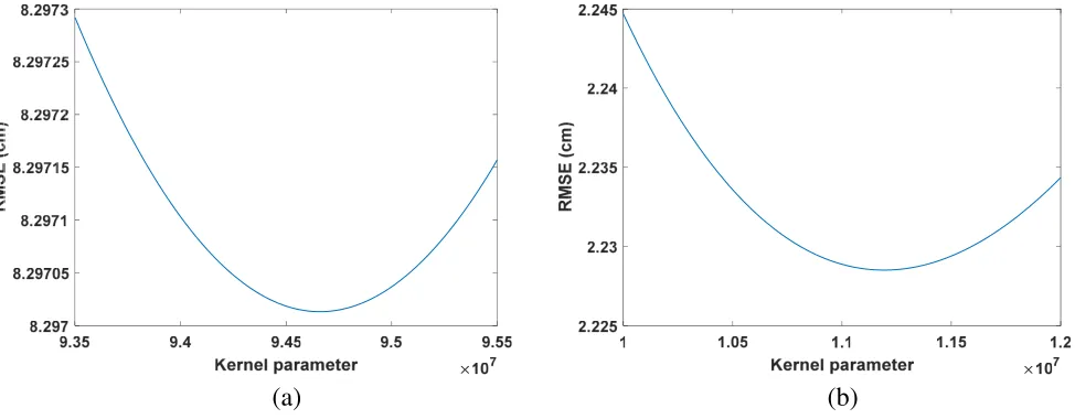
In the training phase of the KELM, γ is the only parameter that needs to be tuned with the knowledge of input data and the number of training samples. Fig. 2 shows that the root mean squared error (RMSE) for the regression changes with the kernel parameter. Whether in thex-direction (cross-range) or z-direction (down-range), the RMSE decreases with increasing kernel parameter, but it will reach a minimum and then increase. Thus, the minimum RMSE occurs when the kernel parameter equals a definite value. According to the value, the training data are trained by the KELM, and the model, which is called modelkelm, is obtained. The ELM model can estimate one parameter at a time, which is similar to the SVM model, or several parameters at one time which is similar to the LS-SVM model. Thus, the ELM-based approach is more convenient and flexible than the SVM-based approach.
(a)
(b)
Based on the testing data, the target location is estimated by modelkelm, and then the degree of matching between the actual and estimated target centers is evaluated qualitatively, as shown in Fig. 3, and quantitatively, as shown in Fig. 4.
0 0.5 1 1.5 2 2.5
Actual values of x-direction (m) 0
0.5 1 1.5 2 2.5
0 0.5 1 1.5 2 2.5 3
Actual values of z-direction (m) 0
0.5 1 1.5 2 2.5 3
(a)
(b)
Figure 3. Estimation values of the (a)x-direction and (b) z-direction versus the actual values.
0 20 40 60 80 100 120 140 160
Sample numbers
-0.6 -0.4 -0.2 0 0.2 0.4 0.6 0.8
SVM LS-SVM KELM
0 20 40 60 80 100 120 140 160
Sample numbers
-1.5 -1 -0.5 0 0.5
SVM LS-SVM KELM
(a)
(b)
Figure 4. Estimation errors between the estimation values and the actual values of the (a)x-direction, and (b)z-direction.
In Fig. 3, the 45-deg diagonal line indicates that the estimated value is equal to the actual value. The round dots represent the estimated values. The closer the round dots are to the diagonal line, the more precise the estimated values are. From Fig. 3, the results show that modelkelm performs well, except for a few samples that are very close to or far away from the wall. The estimated effect of the cross-range is slightly worse than that of the range. The resolution in the down-range direction depends on the signal wideband, while that in the cross-range direction depends on the synthetic aperture. Thus, the KELM approach is affected more by the former. In Fig. 4, the estimated errors of xc are less than
0.05 m, and those of zc are below 0.02 m. The results are compared with the estimated errors of the
the accuracy of the KELM is better than the accuracy of the SVM and worse than the accuracy of the LS-SVM. The estimated accuracy of the LS-SVM is the best; that of the KELM is second; and that of the SVM is third. However, in general, the estimated accuracies of these three approaches are all acceptable and quite suitable for TWRI.
To identify the performance of the KELM in terms of generalization, two targets behind the wall are considered. The simulation scenes are unchanged except for the change in the number of targets. The added target is the same as the original target. The centers of the two targets are (0.45 m, 0.85 m) and (1.66 m, 1.78 m). The locations are different from those in the training data. To avoid the interruption of the two targets, they are placed far apart. The maximum amplitude and the corresponding time corresponding to the different targets are extracted. Through modelkelm, the estimated results are (0.51 m, 0.84 m) and (1.65 m, 2.08 m). From the results, we know that the estimated results are not very good. The reason may be that the signals of the two targets will interfered with each other, although the two targets are placed far apart.
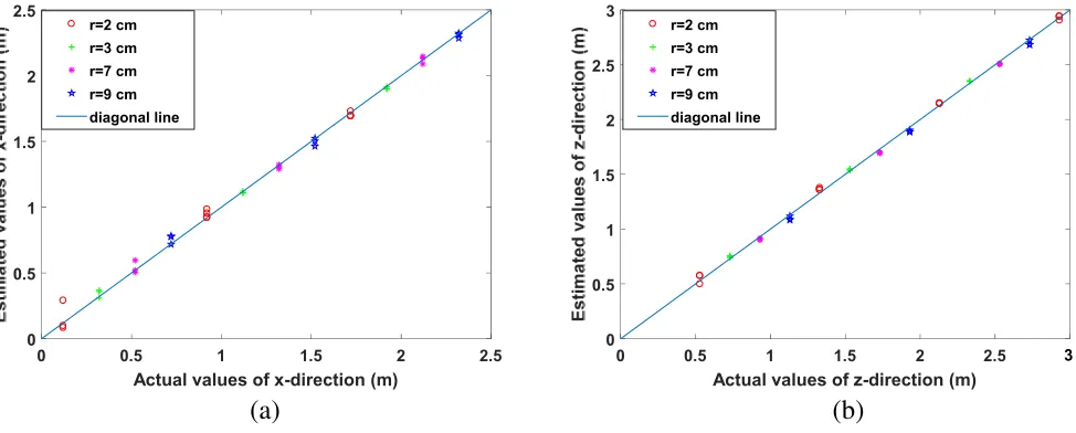
In addition, different radii are discussed. The simulation scenes are unchanged except for the change in the target radius. When the radius is 2 cm,xc of the test data is (0.12 m, 0.92 m, 1.72 m), and
zc is (0.53 m, 1.33 m, 2.13 m, 2.93 m). When the radius is 3 cm, xc of the test data is (0.32 m, 1.12 m,
1.92 m), and zc is (0.73 m, 1.53 m, 2.33 m). When the radius is 7 cm, xc of the test data is (0.52 m,
1.32 m, 2.12 m), and zc is (0.93 m, 1.73 m, 2.53 m). When the radius is 9 cm, xc of the test data are
(0.72 m, 1.52 m, 2.32 m), and zc is (1.13 m, 1.93 m, 2.73 m). All these xc and zc values are from the
test samplings. The maximum amplitude and the corresponding time are extracted. Then, through modelkelm, the estimated results are as shown in Fig. 5. From Fig. 5, we know that the estimated results are almost unaffected when the radii of the targets change.
0 0.5 1 1.5 2 2.5
Actual values of x-direction (m) 0
0.5 1 1.5 2 2.5
r=2 cm r=3 cm r=7 cm r=9 cm diagonal line
0 0.5 1 1.5 2 2.5
Actual values of z-direction (m) 0
0.5 1 1.5 2 2.5 3
r=2 cm r=3 cm r=7 cm r=9 cm diagonal line
(a)
(b)
3
Figure 5. Estimation values of the (a) x-direction and (b) z-direction versus the actual values for different radiuses.
(a)
(b)
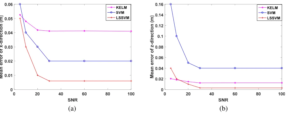
Figure 6. Mean error of the (a)x-direction and (b) z-direction versus the SNR.
operation under noisy circumstances.
In addition, real-time functionality is a crucial and important problem in TWRI. Whether for the KELM, SVM, or LS-SVM approaches, the time needed to locate targets consists of two parts: the training time and the testing time. In this paper, 575 training samples are trained, and the training time is 0.05 s for the KELM approach (which has one training process), 3344.82 s for the SVM approach (which has two training processes), and 1052.0 s for the LS-SVM approach (which has one training process) on a personal computer equipped with a 2.6-GHz processor. The training time for the KELM approach is no more than one second, which is six orders of magnitude shorter than that of the SVM approach or the LS-SVM approach. A total of 156 testing samples are tested, and the testing time is 0.012 s for the KELM approach, 0.351 s for the SVM approach, and 0.297 s for the LS-SVM approach. The testing time for the KELM approach is one order of magnitude shorter than that of the SVM approach or the LS-SVM approach. Although the difference in the testing time is not obvious, the training time for the KELM approach is much shorter than that for the SVM approach or the LS-SVM approach. In the training process, the KELM approach needs to select only the kernel function and determine the appropriate kernel parameter, and does not need to set the number of hidden neurons; hence, it can greatly reduce the amount of time required for optimizing the number. The SVM approach must optimize two parameters, which is time-consuming. Therefore, the KELM approach can locate the target in a few seconds. Compared to the SVM approach and LS-SVM approach, the KELM approach is more suitable for real-time target locating, which is an important requirement in TWRI.
5. CONCLUSIONS
in noisy circumstances. Thus the KELM approach is very suitable for real-time TWRI under unknown wall parameters.
Future works will be aimed at dealing with estimating the target locating of multiple targets and collecting the training data in a real scenario before the detecting task.
ACKNOWLEDGMENT
This work is supported by the National Natural Science Foundation of China [Grant Nos. 61601242, 61601245], Jiangsu Planned Projects for Postdoctoral Research funds [Grant No. 1601150C] and Jiangsu Government Scholarship for Overseas Studies [Grant No. JS-2017-026].
REFERENCES
1. Protiva, P., J. Mrkvica, and J. Machac, “Estimation of wall parameters from time-delay-only through-wall radar measurements,”IEEE Trans. Antennas Propagat., Vol. 59, No. 11, 4268–4278, 2011.
2. Dehmollaian, M. and K. Sarabandi, “Refocusing through building walls using synthetic aperture radar,”IEEE Trans. Geosci. Remot. Sens., Vol. 46, No. 6, 1589–1599, 2008.
3. Solimene, R., F. Soldovieri, G. Prisco, and R. Pierri, “Three-dimensional through-wall imaging under ambiguous wall parameters,”IEEE Trans. Geosci. Remot. Sens., Vol. 47, No. 5, 1310–1317, 2009.
4. Jin, T., B. Chen, and Z. Zhou, “Image-domain estimation of wall parameters for autofocusing of through-the-wall SAR imagery,” IEEE Trans. Geosci. Remot. Sens., Vol. 51, No. 3, 1836–1843, 2013.
5. Soldovieri, F. and R. Solimene, “Through-wall imaging via a linear inverse scattering algorithm,” IEEE Geosc. Rem. Sens. Lett., Vol. 4, No. 4, 513–517, 2007.
6. Li, L. L., W. J. Zhang, and F. Li, “A novel autofocusing approach for real-time through-wall imaging under unknown wall characteristics,” IEEE Trans. Geosci. Remot. Sens., Vol. 48, No. 1, 423–431, 2010.
7. Wang, G. Y., M. G. Amin, and Y. M. Zhang, “New approach for target locations in the presence of wall ambiguities,”IEEE Trans. Aero. Elec. Sys., Vol. 42, No. 1, 301–315, 2006.
8. Ahmad, F., M. G. Amin, and G. Mandapati, “Autofocusing of through-the-wall radar imagery under unknown wall characteristics,” IEEE Trans. on Image Proc., Vol. 16, No. 7, 1785–1795, 2007.
9. Zhang, H. M., Z. B. Wang, Z. H. Wu, F. F. Wang, and Y. R. Zhang, “Real-time through-wall radar image under unknown wall characteristics using LS-SVM-based method,”J. Appl. Remote Sens., Vol. 10, No. 2, 020501-1–8, 2016.
10. Huang, G. B., “An insight into extreme learning machines: Random neurons, random features and kernels,”Cognitive Computation, Vol. 6, No. 3, 376–390, 2014.
11. Huang, G. B., Q. Y. Zhu, and C. K. Siew, “Extreme learning machine: A new learning scheme of feedforward neural networks,”IEEE International Joint Conference on Neural Networks, 985–990, 2004.
12. Huang, G. B., X. J. Ding, and H. M. Zhou, “Optimization method based extreme learning machine for classification,”Neurocomputing, Vol. 74, No. 1, 155–163, 2010.
13. Huang, G. B., H. M. Zhou, X. J. Ding, and R. Zhang, “Extreme learning machine for regression and multiclass classification,” IEEE Trans. on Sys., Man, and Cybernetics, Part B: Cybernetics, Vol. 42, No. 2, 513–529, 2012.
14. Huang, G. B., Y. Lan, and D. H. Wang, “Extreme learning machines: A survey,” Int. J. Mach. Learn. Cyb., Vol. 2, No. 2, 107–122, 2011.