Volume 2009, Article ID 525704,11pages doi:10.1155/2009/525704
Research Article
Introducing Switching Ordered Statistic CFAR Type I in
Different Radar Environments
Saeed Erfanian and Vahid Tabataba Vakili
Electrical Engineering Department, Iran University of Science & Technology (IUST), Narmak, Tehran 16846, Iran
Correspondence should be addressed to Saeed Erfanian,s [email protected]
Received 22 September 2008; Revised 3 December 2008; Accepted 17 February 2009
Recommended by M. Greco
In this paper, a new CFAR detector based on a switching algorithm and OS-CFAR for nonhomogeneous background environments is introduced. The new detector is named Switching Ordered Statistic CFAR type I (SOS CFAR I ). The SOS CFAR I selects a set of suitable cells and then with the help of the ordering method, estimates the unknown background noise level. The proposed detector does not require any prior information about the background environment and uses cells with similar statistical specifications to estimate the background noise. The performance of SOS CFAR I is evaluated and compared with other detectors such as CA-CFAR, GO-CFAR, SO-CFAR, and OS-CFAR for the Swerling I target model in homogeneous and nonhomogeneous noise environments such as those with multiple interference and clutter edges. The results show that SOS CFAR I detectors considerably reduce the problem of excessive false alarm probability near clutter edges while maintaining good performance in other environments. Also, simulation results confirm the achievement of an optimum detection threshold in homogenous and nonhomogeneous radar environments by the mentioned processor.
Copyright © 2009 S. Erfanian and V. Tabataba Vakili. This is an open access article distributed under the Creative Commons Attribution License, which permits unrestricted use, distribution, and reproduction in any medium, provided the original work is properly cited.
1. Introduction
A common routine test in any detection system is to compare the received signal level with a predefined threshold value. If the threshold is crossed, the presence of the signal of interest is declared. In modern radar detection, the decision on target presence or absence is often performed automatically, that is, without the visual intervention of the radar operator. When the threshold is a fixed value, the false alarm rate will increase intolerably (i.e., beyond a level that the computer of an automatic detector can handle) as the interference power varies. In this situation, aconstant false alarm rate(CFAR) algorithm with an adaptive threshold is required to keep the false alarm rate constant.
In a radar receiver, after amplitude detection, the backscattered signal is sampled in range and/or Doppler and a one- or two-dimensional reference window is formed. The detection in radar means existence or nonexistence of a target in the middle cell of a reference window or a cell under test (CUT). The noise and clutter background is estimated by processing the output from neighbouring cells. A
well-known group for noise estimation is mean-level detectors such as cell averaging CFAR (CA) [1]. Unfortunately because of differences in environmental conditions such as change in clutter edge, multiple targets, or jamming the target detection will be corrupted. As solutions for these problems, various CFAR schemes are proposed. A few examples are the greatest of CFAR (GO-CFAR), the smallest of CFAR (SO-CFAR), order statistics CFAR (OS-CFAR), the excision cell-averaging CFAR (EXCA-CFAR), and the excision of the greatest of CFAR (EXGO-CFAR) [2,3]. Each of these schemes has advantages and disadvantages but none of them shows considerably good performance in all types of environments. However, the processors which use ordering have better performance than mean levels.
detector is based on comparing cells with scaled CUT to set the cells with the same statistical specifications in two groups. By counting the number of cells in each group and finding the group with more cells, estimation of background noise will be performed [4]. In this paper after describing the SOS CFAR I algorithm in Section 2, mathematical and related probabilities of detection and false alarms are presented in
Section 3. In Section 4the performance and simulation of the SOS I processor in homogeneous and nonhomogeneous environments will be analysed, and in the last section the results are presented.
2. Description of SOS CFAR I Method
In this paper, it is assumed that the CFAR processor’s inputs are range samples (range cells) which are received from the square law detector and are saved into a tapped delay line of length 2N + 1. The 2N samples correspond to reference cells Xi surrounding the test cellX0. The SOS I detector block diagram is provided in Figure 1. Here, single pulse detection and a Rayleigh fading model are assumed for fluctuating targets corresponding to Swerling I in single pulse processing. For a homogeneous noise pulse clutter level, the in-phase I and quadrature Q input signals are assumed independent and identically distributed (iid) Gaussian random variables with zero mean. Consequently, the output samples of the square law detector are also iid R.V.s with an exponential distribution [6, 7]. Thus, the probability density function (PDF) of theith cell is
fXi
xi
=1
λe
−xi/λ, x
i≥0,λ≥0, 1≤i≤2N, (1)
in whichXis are 2Nwindow samples (excluding the CUT),
and λ is the total background clutter-plus-thermal noise power. If a cell contains thermal noise thenλ = λ0 = 2η, and if it consists of clutter then λ = λc = 2η(1 +σc). If
a cell consists of multiple (not primary) targets then in (2)
λ=λI=2η(1 +σI). Alsoσcis the ratio of clutter’s power to
the noise power, andσIis the ratio of multiple targets’ power
to the noise.
Target detection in CUT is carried out by estimating the 2Nreference window cells that surround it. The PDF of CUT is the same as (1) in the case of thermal noise withλ=λ0= 2η, and in the case of primary (main) target it will be in the form of (2) withλ=λs=2η(1 +σs) whileσsis the ratio of
the signal power to the noise power:
fX0
x0
=1
λe
−x0/λ, x
0≥0,λ≥0. (2)
InFigure 1the SOS I detector first divides reference samples into twoS1 andS0 groups by comparing them with scaled
X0 with α < 1. This is a criterion for finding samples with the same specification. In other words, it implies collecting samples with the same amplitude in one group. Next, estimation of the background noise will be done based onS0group or 2Nsamples of reference window. The manner of selection is based on comparing the number ofS0group samples (n0) with an integer threshold NT. If n0 is more
Input samples Square law detector
X2N · · · X0 · · · X1
Y
· · ·
N Xi< αX0
Saved inS0(n0) Saved inS1(2N−n0) n0> NT N
Y
Estimation by 2Ncells Estimation
byS0
Figure1: Block diagram of SOS CFAR I.
thanNT, background noise will be estimated only with the
S0 samples, but if n0 is less than NT, similar to SCFAR
[8,9], all the samples of the reference window are selected. In both cases, background noise estimation is obtained from one of the ordered samples of S0 or the whole reference window. The range samples in both groups are first ordered according to their magnitudes, and the estimation is taken to be the kth largest sample. Also, NT is selected based
on detector requirements and environment conditions. This process gives the detector an ability to suppress the masking effect caused by interfering targets and clutter edge. Thus, the algorithm will be carried out in the following two steps.
(i) 2N cells in the reference window will be compared with the scaled CUT byα(α <1). If a cell value is less than
αX0it will be saved in groupS0, otherwise it will be saved in
S1as in
Xi S1
≥
<
S0
αX0, i=1, 2,. . ., 2N. (3)
(ii) If the number of samples saved in group S0 is n0, then the target will exist in CUT according to the following conditions:
IfX0> β0X(k0)=β0Z0, whenn0> NT, (4)
or
IfX0> β1X(k1)=β1Z1, whenn0≤NT, (5)
whereβ0andβ1are constants for achieving the desired false alarm probability, andNTis the threshold integer. Also, in (4)
and (5)k0andk1are rounded (g0×n0) and (g1×2N) where
g0andg1are parameters between 0 and 1. By adjustingg0and
g1, the order of each selected group is achieved.
Inequalities (4) and (5) mean that SOS CFAR I switches between the sample setS0and whole reference, depending on the value ofn0. For example, if the number of samples which have a value lower than the scaled CUT (and are saved inS0) is more than the preset thresholdNT, noise level estimation
S0and selectingk0th of them; but if the number of samples which have a value lower than the scaled CUT is less than the considered threshold, the noise level estimation is carried out by ordering homogeneous saved samples in the whole reference window and selectingk1th of them. This type of processing by the SOS CFAR I processor means selecting an optimized threshold of detection in homogeneous and nonhomogeneous environments.
3. Mathematical Analysis of SOS CFAR I
Switching Ordered Statistics type I CFAR detector incor-porates a switching method to estimate the total noise power. Such a detector is specifically tailored to provide good estimates of the noise power with an exponential PDF. In this section we analyse the performance of the SOS CFAR I processor in a homogeneous background as well as in regions of clutter transitions and in multiple target environments. We obtain closed-form performance expressions in each case.
3.1. Homogeneous Environment. Considering the algorithm described in Section 2and considering the existence of n0 samples inS0 and 2N−n0 samples inS1, and by referring to (4) and (5), the detection probability of SOS CFAR I is
Pd=Pd0+Pd1, (6)
in which Pd0 is the probability of detection when S0 is
selected, and Pd1 is the probability of detection when the
whole reference window is selected. If we assume presence of a target,H1, we have
Pd=P
whenS0 is selected|H1
+Pwhen the whole reference window is selected|H1
, (7)
which is equal to
Pd
=Probability of savingNT+ 1≤n0≤2N
samples in S0
×Probability thatX0 is more than
β0Z0
+ Probability of saving0≤n0≤NT
samples in S0
×Probability thatX0 is more than
β1Z1
.
(8)
Therefore, the probability of detection when the whole reference window is selected is
Pd1=
NT
n0=0
Ps×P
X0> β1Z1|H1
, (9)
where Ps is the probability that there are (based on (8))
exactlyn0noise samples inS0and is equal to
PS=EX0
⎧ ⎨ ⎩ ⎛ ⎝2N
n0
⎞ ⎠Pn0
0
x0
1−P0
x0
2N−n0
⎫ ⎬
⎭. (10)
P0(x0) is the probability that a noise sample belongs to S0, which is computed as
P0
x0
=PXi< αX0
=
αx0
xi=0 fXi
xi
dxi
=
αx0
xi=0
1
λe
−xi/λd
xi
=1−e−(α/λ)x0.
(11)
In (11), it is assumed that the samples are independent, the window samples contain thermal noise and the CUT contains signal [10]. By using (A.1) in Appendix A, (10) becomes
PS=
⎛ ⎝2N
n0
⎞ ⎠n0
i=0
⎛ ⎝n0
i ⎞
⎠ (−1)i
α2N−n0+i
1 +σs
+ 1. (12)
In (9),Z1is the random variable obtained from the ordering of 2N noise samples in the reference window and selecting
k1of them as an estimation of noise in the case ofn0 < NT.
Now, if as (5) we considerZ1=X(k1), then the PDF ofZ1is given by [11]
fK1(z1)=K1
⎛ ⎝2N
K1
⎞
⎠e−z1/λ2N−K11−e−z1/λK1−11
λe
−z1/λ.
(13)
Therefore by referring toAppendix B,
PX0> β1Z1|H1
= (2N)!
2N−k1
!
k1−1
m=0
(−1)m
m!k1−m−1
!
1 2N−k1+m+β1/
1 +σs
.
(14)
For calculating the probability of detection when only the samples inS0are selected, similar to (9), one has
Pd0=
2N
n0=NT+1 Ps×P
X0> β0Z0|H1
, (15)
wherePSwas calculated in (10). Therefore same as (14),
PX0> β0Z0|H1
= n0!
n0−k0
!
k0−1
m=0
(−1)m
m!k0−m−1
!
1
n0−k0+m+β0/
1 +σs
.
M 2N−M Whole reference
m n0−m M−m 2N−n0−(M−m)
S0 S1
Figure2: Position of noise samples in nonhomogeneous environ-ment.
By using (9) and (15), the result will be
PSOS I
d
NT,α,β0,β1,g0,g1
=
NT
n0=0
⎛ ⎝2N
n0
⎞ ⎠n0
i=0
⎛ ⎝n0
i ⎞
⎠ (−1)i
α2N−n0+i
1+σs
+1
(2N)!
2N−k1
!
×
k1−1
m=0
(−1)m
m!k1−m−1
!
1 2N−k1+m+β1/
1+σs
+ 2N
n0=NT+1 ⎛ ⎝2N
n0
⎞ ⎠n0
i=0
⎛ ⎝n0
i ⎞
⎠ (−1)i
α2N−n0+i
1+σs
+1
n0!
n0−k0
!
×
k0−1
m=0
(−1)m
m!k0−m−1
!
1
n0−k0+m+β0/
1+σs
.
(17)
Also, using (17) and settingσsequal to zero, the probability
of occurrence of a false alarm can be determined as
PSOS I fs
NT,α,β0,β1,g0,g1
=
NT
n0=0
⎛ ⎝2N
n0
⎞ ⎠n0
i=0
⎛ ⎝n0
i ⎞
⎠ (−1)i
α2N−n0+i
+ 1
(2N)!
2N−k1
!
×
k1−1
m=0
(−1)m
m!k1−m−1
!
1 2N−k1+m+β1
+ 2N
n0=NT+1 ⎛ ⎝2N
n0
⎞ ⎠n0
i=0
⎛ ⎝n0
i ⎞
⎠ (−1)i
α2N−n0+i
+1
n0!
n0−k0
!
×
k0−1
m=0
(−1)m
m!k0−m−1
! 1
n0−k0+m+β0.
(18)
3.2. Nonhomogeneous Environment. Considering the algo-rithm described inSection 2, it is assumed that in a reference window with a size equal to 2N, there are M interfering samples and 2N−Mthermal noise samples, andS0contains
minterfering samples andn0−mthermal noise samples as illustrated inFigure 2. Assuming that there aren0samples in
S0and 2N−n0samples inS1and by referring to (4) and (5), the detection probability in SOS I will be as follows.
For M interfering samples that appear in the CFAR window, the probability that exactlymof them are stored in
S0is
q1s=
⎛
⎝M
m ⎞
⎠P
0
X0
m
1−P0
X0
M−m
. (19)
For 2N−Mthermal noise samples that appear in the CFAR window, the probability that exactlyn0−mof them are stored inS0is [8]
q0s=
⎛
⎝2N−M
n0−m
⎞
⎠P0X0n0−m
1−P0
X0
2N−M−(n0−m)
.
(20)
Therefore, the probability that there are exactlyminterfering samples andn0−mthermal noise samples inS0is
Qs=q0s×q1s
=EX0
min(M,n0)
m=m1
⎛
⎝2N−M
n0−m
⎞ ⎠ ⎛
⎝M
m ⎞
⎠P0X0n0−m
×1−P0
X0
2N−M−(n0−m)
×P0m
X0
1−P0
X0
M−m
.
(21)
Here, the probability of existence of a sample with thermal noise in theS0group is determined by (11). Also, the probability of existence of a sample with interference noise in
S0group according to (3) is
P0
X0
=PXi< αX0
=
αx0
xi=0 fXi
Xi
dxi
=
αx0
xi=0
1
λ1e −xi/λId
xi
=1−e−(α/λI)x0.
(22)
Therefore, with the help of (11) and (22) and referring to
Appendix C, (21) will be
Qs=
min(M,n0)
m=m1
⎛
⎝2N−M
n0−m
⎞ ⎠ ⎛
⎝M
m ⎞ ⎠
×
n0−m
t=0
m
q=0
(−1)t+qn0−m
t
m
q
1+N(1+σs)α+(M−m+q)
(1+σs)/(1+σI)
α,
(23)
the probability of detection in the case of interfering targets will be
PdSOS I
NT,α,β0,β1,g0,g1
=
NT
n0=0
Qs×P
X0> β1Z1|H1
+ 2N
n0=NT+1 Qs×P
X0> β0Z0|H1
.
(24)
Referring toAppendix D, in the case of a nonhomogeneous environment, one has
PX0> β1Z1|H1
= β1
1 +σs
2N
i=k1
p2
L=p1
⎛
⎝2N−M
L ⎞ ⎠ ⎛
⎝ M
i−L ⎞ ⎠
×
L
j1=0
i−L j2=0
L j1
i−L j2
(−1)j1+j2
2N−M−L+β1/
1 +σs
+j1+Q/
1 +σI
,
(25)
whereQdenotes (j2+M−i+L). And with the same procedure in theS0group,
PX0> β0Z0|H1
= β0
1 +σs
2N
i=k0
t2
L=t1
⎛ ⎝n0−m
L ⎞ ⎠ ⎛
⎝ m
i−L ⎞ ⎠
×
L
j1=0
i−L
j2=0
L j1
i−L j2
(−1)j1+j2
n0−m−L+β0/
1 +σs
+j1+C/
1 +σI
,
(26)
whereCdenotes (j2+m−i+L) andt1 andt2are equal to max(0,i−m) and min(i,n0−m).
Now we investigate the performance of the SOS I processor when the reference window contains a clutter edge. First, consider the special case where CUT is not from the clutter region. Also similar to the multiple targets case, it is assumed that in a reference window with a size equal to 2N, there areMsamples from clutter and 2N−Mthermal noise samples, andS0containsmsamples from clutter andn0−m thermal noise samples. First, the probability of existence of a sample with thermal noise in theS0group according to (3) was calculated in (11). Also, the probability of existence of a sample with clutter noise in theS0group according to (22) is
P0
X0
=PXi< αX0
=
αx0
xi=0 fXi
xi
dxi
=
αx0
xi=0
1
λCe
−xi/λCd
xi
=1−e−(α/λC)x0.
(27)
Here with the help of (23), (24), (25), and (26) and consideringσs →0 andσI → σC, thePSOS If a will be
PSOS I
f a
NT,α,β0,β1,g0,g1
=
NT
n0=0
Qs×P
X0> β1Z1|H0
+ 2N
n0=NT+1 Qs×P
X0> β0Z0|H0
,
(28)
where
PX0> β1Z1|H0
=β1 2N
i=k1
p2
L=p1
2N−M L
M i−L
×
L
j1=0
i−L
j2=0
L j1
i−L j2
(−1)j1+j2
2N−M−L+β1+j1+Q/
1 +σC
, (29)
PX0> β0Z0|H0
=β0 2N
i=k0
t2
L=t1
n0−m
L
m i−L
×
L
j1=0
i−L
j2=0
L j1
i−L j2
(−1)j1+j2
n0−m−L+β0+j1+C/
1 +σC
,
(30)
where
Qs=
min(M,n0)
m=m1
2N−M n0−m
M m
×
n0−m
t=0
m
q=0
(−1)t+qn0−m
t
m
q
1 +Nα+ (M−m+q)1/1 +σC
α.
(31)
Now if CUT is from the clutter region, after substitutingσI=
σs,β0,β1, andαbyσC,β0/(1 +σc),β1/(1 +σc), andα(1 +σc)
in (23), (24), (25), (26), and also
PX0> β1Z1|H0
= β1 1 +σC
2N
i=k1
p2
L=p1
⎛
⎝2N−M
L ⎞ ⎠ ⎛
⎝ M
i−L ⎞ ⎠
×
L
j1=0
i−L
j2=0
L j1
i−L j2
(−1)j1+j2
2N−M−L+β1/
1 +σC
+j1+Q/
1 +σC
.
(32)
PX0> β0Z0|H0
= β0 1 +σC
2N
i=k0
t2
L=t1
⎛ ⎝n0−m
L ⎞ ⎠ ⎛
⎝ m
i−L ⎞ ⎠
×
L
j1=0
i−L
j2=0
L j1
i−L j2
(−1)j1+j2
n0−m−L+β0/
1 +σC
+j1+C/
1 +σC
,
−20
−18
−16
−14
−12
−10
−8
−6
−4
−2 0
log
10
(
Pfa
)
0 2 4 6 8 10
β0=β1
OS,K=N=9 OS,K=17
SOS,NT=N,α=0.9, g0=g1=0.9
SOS,NT=N,α=0.1, g0=g1=0.9
Simulation: SOS,NT=N,α=0.1, g0=g1=0.9, data=20000
SO
GO CA
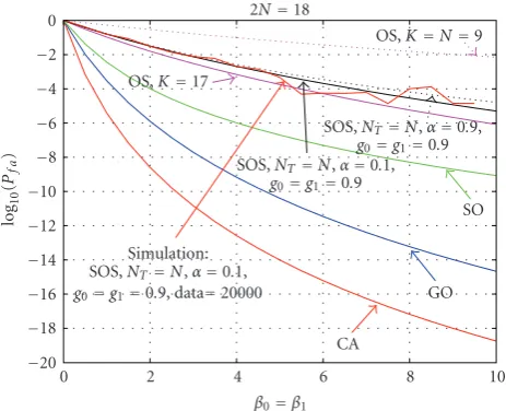
2N=18
Figure3: False alarm probability of the CA, GO, SO, OS (k=N=9 andk=17), and SOS CFAR I processors for 2N=18.
where
Qs=
min(M,n0)
m=m1
⎛
⎝2N−M
n0−m
⎞ ⎠ ⎛
⎝M
m ⎞ ⎠
×
n0−m
t=0
m
q=0
(−1)t+qn0−m
t
m
q
1 +N1 +σC
α+ (M−m+q)α.
(34)
4. Studying SOS CFAR I in Different Conditions
The performance of the Switching Ordered Statistic CFAR I processor algorithm, according to (11), is a function of
β0,β1,NT,α,g0, andg1. These parameters should be tuned such that the SOS CFAR I processor has minimum CFAR loss when operating in a homogeneous environment. Provided that there are only noise samples within the CFAR window, almost all reference samples will be stored to S0 if the test cell contains a target return signal with substantial SNR. The SOS CFAR I processor then tends to switch toS0, and the threshold multiplierβ0 andg0 are employed with high probability. In order to minimise the CFAR loss in this situation,g0(k0) should be set as close as possible to the order of OS CFAR (corresponding to the false alarm probability of interest). If the test cell contains no target signal, far fewer reference samples are sorted toS0. The whole CFAR window and orderingg1(k1) are then employed with high probability. In order to maintain the false alarm rate as that of the OS-CFAR, g1 (k1) should also be set as close as possible to k of the OS. Therefore, a reasonable choice is g0 = g1. Also, for preventing complexity,β0 =β1 is considered, although different values forβ0 andβ1 could be considered for the future. The setting of the SOS CFAR I parameters for the case
g0=g1andβ0=β1are briefly discussed in this section [8]. In order to detect targets near a clutter edge, the threshold integer should be approximately equal to or smaller than
−6.5
−6
−5.5
−5
−4.5
−4
−3.5
−3
log
10
(
Pfa
)
0 0.2 0.4 0.6 0.8 1
α β=5
β=6 β=7 β=9
β=11
β=13
Simulation: β=6 and data=38000
Figure4: False alarm probability of the SOS CFAR I processor for differentβ0=β1in terms ofα.
the half window size, that is, NT ≤ N. An SOS CFAR I
processor with a smaller NT can tolerate a greater number
of interference samples, but in a homogeneous environment it suffers from more CFAR loss compared to the CA-CFAR. Here CFAR loss, based on [12, 13], is defined as the additional SNR the CFAR processor requires in order to achieve the same detection probability at a given false alarm rate.
The curves in Figure 3are the false alarm probabilities (Pf a) for a reference window with the size 2N=18 for SOS I,
withNT =N =9,β0=β1,g0=g1=0.9,α=0.1, andα= 0.9, CA, GO, SO, and OS (withk=N=9 andk=17) in a homogeneous environment. It is seen that in a homogeneous environment, onlyPf aof OS withk=N =9 is worse than
SOS I. For verifying the theoretical results, the performance of SOS I withNT = N = 9,β0 = β1,g0 = g1 = 0.9, and
α=0.1 has been simulated by the Monte Carlo method for about 20 000 data for each point. As it is shown, this curve is compatible with the analytical curve.
InFigure 4,Pf aof the performance of SOS I processor
in a homogeneous environment with 2N = 18,NT = N,
andg0 = g1 = 0.9 have been plotted forα and different values of β0 = β1. It is clear that by increasing β0 =
β1,Pf ais decreasing. Also, it is seen that in all cases withα
larger than 0.4 and withβ0 =β1,Pf ais increasing. Also in
Figure 4the curve for β = 6 has been simulated with the Monte Carlo method for about 38000 data for each point which is compatible with the analytical curve with the same parameters.
InFigure 5,Pf aof the SOS I processor in a homogeneous
environment with 2N =18,β0 =β1 =9, andα=0.5 and for differentNT values have been plotted forg0 = g1. It is clear that by increasingNT,Pf ais decreasing.
The probability of the occurrence of a false alarm by the SOS I detector in a homogeneous environment based on differentNT andαvalues have been plotted forg0 = g1in
−7
−6
−5
−4
−3
−2
−1 0
log
10
(
Pfa
)
0.1 0.2 0.3 0.4 0.5 0.6 0.7 0.8 0.9 1 g0=g1
NT=3 NT=6
NT=15 NT=8 2N=18,β0=β1=9,α=0.5
Figure5: Comparison ofPf ain SOS I with differentNTin terms of
g0=g1in homogeneous environment with 2N =18.
−7
−6
−5
−4
−3
−2
−1 0
log
10
(
Pfa
)
0.1 0.2 0.3 0.4 0.5 0.6 0.7 0.8 0.9 1 g0=g1
NT=6,α=0.4
NT=3,α=0.1
NT=15,α=0.9 NT=8,α=0.5 2N=18,β0=β1=9
Figure6: Comparison ofPf afor SOS I proceαsor in homogeneous environment in terms ofg0=g1and some differentNTandαwith 2N=18.
and increasingα,Pf a is decreasing. Also it is clear that by
increasing bothNTandαparameters,Pf ais again decreasing.
Now, inFigure 7, the detection probability of the SOS I detector in a homogeneous environment in comparison with the optimum detector, CA, GO, SO, and OS (with
k = N = 9 and k = 17) and for Pf a = 10−5, has
been drawn. The optimum detector sets a fixed threshold to determine the presence of a target under the assumption that the total homogeneous noise power is known a priori [10]. Considering the loss detection, it is seen that the SOS I processor with NT = N,α = 0.1,β0 = β1 = 9, and
g0=g1=0.9 has inherent detection loss in the homogeneous environment which is more than CA and GO but is less than SO and OS (k = N = 9). Also, this figure shows that by increasing the order of OS tok=17, its detection loss will be
0 0.1 0.2 0.3 0.4 0.5 0.6 0.7 0.8 0.9 1
Pd
0 5 10 15 20 25 30
SNR (dB) SOS,NT=N,α=0.1,g0=g1=0.9
CA GO
Optimum Simulation: SOS, NT=N,α=0.1, g0=g1=0.9,
data=20000
SO OS,K=N=9 2N=18,Pf a=10−5
Figure7: Comparison ofPdfor CA, GO, SO, OS (k=N =9 and
k=17), and SOS I processors (2N=18 andPf a=10−5).
0 0.1 0.2 0.3 0.4 0.5 0.6 0.7 0.8 0.9 1
Pd
0 5 10 15 20 25 30
SNR (dB)
NT=7,g0=g1=0.983 NT=8,g0=g1=0.938 NT=15,g0=g1=0.9
Optimum
2N=18,β0=β1=9,α=0.5,Pf a=10−5
Figure8: Comparison ofPdfor SOS I with differentNTandg0=g1 (2N=18 andPf a=10−5).
less than the SOS I detector with the mentioned parameters. In fact, with the help ofFigure 3, increasingkin OS causes less detection loss but a higher probability of false alarm. For better comparison, thePdof SOS I is achieved by the Monte
Carlo simulation with 20000 data for each point. AsFigure 7
shows, the result of the Monte Carlo simulation is the same as the analysis result ofSection 3.
InFigure 8the detection probability of the SOS I detector in a homogeneous environment with different values of
NT,g0 =g1and forPf a =10−5,β0 =β1 =9, andα =0.5 has been plotted. The result shows that with greaterNT and
smallerg0=g1, it has less detection loss.
−12
−10
−8
−6
−4
−2 0
log
10
(
Pfa
)
0 2 4 6 8 10 12 14 16 18
Number of cluster cells SOS,NT=N,α=0.1,g0=g1=0.9
SO
OS,K=N CA
GO
S,NT=N,α=0.1 OS,K=17 2N=18, CNR=10 dB
Figure9: Comparison ofPf afor CA, GO, SO, OS (k=N=9), and SOS I processors (2N=18 and CNR=10 dB).
0 0.1 0.2 0.3 0.4 0.5 0.6 0.7 0.8 0.9 1
Pd
0 5 10 15 20 25 30
SNR (dB) SOS,NT=N,α=0.1,g0=g1=0.9
Simulation: SOS, NT=N,α=0.1, g0=g1=0.9,
data=10000 Optimum
SO
OS,K=N&K=17 CA GO 2N=18,I=1, INR=SNR,Pf a=10−5
Figure10: Comparison of Pdof SOS I by CA, GO, SO, and OS (k=Nandk=17) in the case of one multiple targets (INR=SNR) forPf a=10−5and 2N=18.
equal to 10 dB, Pf a = 10−5, and 2N = 18. It is known
that in the presence of clutter edge, the GO processor has the lowest probability of false alarm and is followed by CA, S withNT = N,α = 0.1, OS (k = 17), and SOS I with
NT=N,α=0.1, andg0=g1=0.9. It is clear fromFigure 9 that OS (k = N = 9) and SO are after it, and also GO has the best performance among all the CFAR processors in the presence of clutter.
The presence of multiple targets is another case in studying the SOS I processor. InFigure 10 one interfering target with interference to noise ratio (INR) equal to SNR and the size of reference window 2N = 18 for CA, GO, SO, OS (k = N = 9 and k = 17), and SOS I processors
0 0.1 0.2 0.3 0.4 0.5 0.6 0.7 0.8 0.9 1
Pd
0 5 10 15 20 25 30
SNR (dB) SOS,NT=N,α=0.1,
g0=g1=0.9
Optimum
S,NT=N,α=0.1 SO
OS,K=15 OS,K=N
OS,K=17 CA GO
2N=18,I=3, INR=2SNR,Pf a=10−5
Figure11: Comparison ofPdof SOS I by CA, GO, SO, and OS (k =N =9,k = 15, andk = 17) in the case of three multiple targets (INR=2SNR) forPf a=10−5and 2N=18.
0 0.1 0.2 0.3 0.4 0.5 0.6 0.7 0.8 0.9 1
Pd
0 5 10 15 20 25 30
SNR (dB) I=5, INR=3SNR
I=5, INR=SNR
I=7, INR=5SNR
Optimum
NT=N,α=0.1β0=β1=9,g0=g1=0.9
2N=18,Pf a=10−5
Figure12: Comparison ofPdof SOS I withNT=N,α=0.1,β0=
β1 = 9, andg0 = g1 = 0.9 in multiple targets environment for 2N =18 andPf a=10−6.
with considered parameter in this figure and forPf a =10−5
are considered. As the result shows, SOS I has the best performance. By increasing the order of OS, its performance will become constant and will be equal to SO which have less
Pd in terms of SOS I with considered parameters. The result
of the Monte Carlo simulation for 10000 data for each point is also confirmed by the result of theoretical analysis. It is noticeable that if data numbers for each point increase, the Monte Carlo simulation will have better compatibility with theoretical results.
0 10 20 30 40
Po
w
er
(d
B
W
)
0 10 20 30 40 50 60
Range
SO GO
CA 2N=18,Pf a=10−5
(a)
0 10 20 30 40
Po
w
er
(d
B
W
)
0 10 20 30 40 50 60
Range OS,K=17
OS,K=N=9
SOS,NT=N,α=0.1,β0=β1=9,g0=g1=0.9
(b)
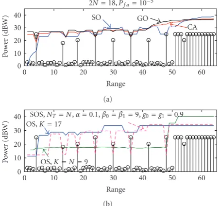
Figure13: Detection thresholds of CA, GO, SO, OS (k=N=9 and 17), and SOS I (NT =N,α=0.1,β0=β1=9, andg0=g1=0.9) in worse case (2N=18 andPf a=10−5).
figure. The results show that SOS I has the best performance and following it, there is the SO detector and then OS with
k = N = 9. If k increases (e.g., k = 15 and k = 17 are considered), its performance decreases and even will be worse than the CA detector. Also,Figure 11shows that the
Pd of S with NT = N and α = 0.1 in the case of three
multiple targets and INR = 2SNR will be reduced, and its performance is less than SOS I and SO with on SNR of more than 16 dB.
InFigure 12,Pd for the case of five and seven multiple
targets and different INR values is shown. The results show thatPd of this detector for I = 5 and INR = 3SNR is the
highest. If in this case INR decreases, then Pd for an SNR
higher than 16 dB will decrease.I=7 and INR=5SNR have the lowestPd. In this figure, 2N=18,NT =N,α=0.5,β0=
β1=9,g0=g1=0.9, andPf a=10−5.
The detection threshold simulation is carried out using Matlab software in the presence of clutter and multiple targets. In Figures13(a)-13(b), there are 8 targets in ranges 4, 13, 18, 24, 30, 36, 42, and 48 with the SNR values mentioned in the figure. Considering the cases with the reference window’s sizes equal to 2N = 18 andPf a =10−5
and fromFigure 13(a), the CA processor can only detect the first target while GO can detect the 1st, 4th, and 6th targets and SO can detect the 1st, 4th, 6th, and 8th targets. From
Figure 13(b), OS (k =N =9) can detect all the targets, OS (k =17) detects only the 1st, and SOS with the mentioned parameters detects all the targets except the 7th target.
InFigure 14the effect of changing SOS I parameters on its detection threshold has been analysed. As seen, SOS I with
β0 = β1 = 149 has the worst detection level and misses many targets. In general, asFigure 14shows, ifαdecreases, the processor has a better estimation level.
0 5 10 15 20 25 30 35 40 45 50
Po
w
er
(d
B
W
)
0 10 20 30 40 50 60 70
Range
α=0.5,β0=β1=149,g0=g1=0.3 α=0.9,β0=β1=10,g0=g1=0.9
α=0.5,
β0=β1=8.95,g0=g1=0.9
α=0.1,β0=β1=8.71, g0=g1=0.9
2N=18,Pf a=10−5,NT=N
Figure14: Detection thresholds of SOS I with different parameters in worst case for 2N=18 andPf a=10−5.
Considering the result of this section, we see that select-ing largerβ0 =β1andg0 =g1versus smallerαandNT =N
causes lessPf a in a homogeneous environment and better
performance forPdin homogeneous and nonhomogeneous
environments, but results in worsePf a in the presence of
clutter edge. Therefore, to have the best performance in var-ious radar environments, suitable parameters, as discussed, should be selected to achieve optimal performance. Also, as the results above and equations inSection 3show, increasing
NT causes the performance of SOS I to become similar to
OS; since, based on (17) and (18), in this case all the samples in the reference window are chosen for background noise estimation (which is based on an Ordered Statistic process), therefore its performance will be near to OS.
5. Conclusions
Appendices
A.
By using (11),PSin (10) can be calculated as follows:
PS=EX0
2N n0
Pn0
0
x0
1−P0
x0
2N−n0
=
∞
x0=0
2N n0
Pn0
0
x0
1−P0
x0
2N−n0
fX0
x0 dx0 = ∞
x0=0
2N n0
1−e−(α/λ)x0n0e−(α/λ)x02N−n0 1
λSe
−x0/λSdx
0 = 1 λS 2N n0 ∞
x0=0
e−((α/λ)(2N−n0)+1/λS)x0
× n0 i=0 n0 i
−e−(α/λ)x0idx
0 = 1 λS 2N n0 n0 i=0 n0 i
(−1)i∞ x0=0
e−((α/λ)(2N−n0+i)+1/λS)x0dx
0 = 1 λS 2N n0 n0 i=0 n0 i
(−1)i 1
(α/λ)2N−n0+i
+ 1/λS
= 2N n0 n0 i=0 n0 i (−1)i
α2N−n0+i
1 +σs
+ 1.
(A.1)
B.
By employing (12), for calculatingP(X0 > β1Z1 | H1), one has [8]
Px0> β1Z1|H1
=
∞
z1=0
∞
x0=β1Z1
1
λ1 +σs
e−x0/λ(1+σs)dx
0fK1
z1 dz1 = ∞
z1=0
e−(β1/λ(1+σs))z1f
K1
z1
dz1
=Mz1
β
1
λ1 +σs
,
(B.1)
whereMZ1(u) is the moment generating function ofZ1and
gives
MZ1(u)=
∞
z1=0
e−uz1K
1 2N K1
e−z1/λ2N−K1
×1−e−z1/λK1−11
λe
−z1/λdz
=K1
2N K1 1 λ ∞
z1=0
1−e−z1/λK1−1
×e−(u+(2N−K1+1)/λ)z1dz
1
=K1
2N K1 1 λ ∞
z1=0
K1−1
m=0
K1−1
m
−e−z1/λm
×e−(u+(2N−K1+1)/λ)z1dz
1
=K1
2N K1 1 λ
K1−1
m=0
K1−1
m
(−1)m
×
∞
z1=0
e−(u+(2N−K1+1)/λ+m/λ)z1dz
1
=K1
2N K1 1 λ
K1−1
m=0
K1−1
m
(−1)m
× 1
u+2N−K1+ 1
/λ+m/λ.
(B.2)
Therefore by settingu=β1/λ(1 +σs) in (B.2),
PX0> β1Z1|H1
= (2N)!
2N−K1
!
×
K1−1
m=0
(−1)m
m!K1−m−1
!
1
β1/
1+σs
+2N−K1+1+m
.
(B.3)
C.
Referring to (11) and (22),QSin (21) can be calculated in the
following manner:
Qs=EX0
min(M,n0)
m=m1
2N−M n0−m
M m P0 X0
n0−m
×1−P0
X0
2N−M−(n0−m)
×P0
X0
n0−m
1−P0
X0
M−m
=
∞
X0=0
min(M,n0)
m=m1
2N−M n0−m
M m P0 X0
n0−m
×1−P0
X0
2N−M−(n0−m)
×P0
X0
m
1−P0
X0
M−m
fX0
x0
dx0
= min(M,n0)
m=m1
2N−M n0−m
M m × ∞
x0=0
1−e−(α/λ)x0n0−me−(α/λ)x02N−M−(n0−m)
×1−ve−(α/λI)x0me−(α/λI)x0M−m1
λSe
−x0/λSdx
= min(M,n0)
m=m1
2N−M n0−m
M m
×
∞
x0=0
1
λSe
−(((2N−M−(n0−m))/λ)α+((M−m)/λI)α+1/λS)x0
×
n0−m
t=0
n0−m
t
(−1)te−((α/λ)t)x0
×
m
q=0
m
q
(−1)q
e−((α/λI)q)x0dx
0
= min(M,n0)
m=m1
2N−M n0−m
M m
× 1
λS n0−m
t=0
m
q=0
n0−m
t
m q
(−1)t+q
×
∞
x0=0
e−(((2N−M−(n0−m))/λ)α+((M−m)/λI)α+1/λS+(t/λ)α+(q/λI)α)x0dx
0
= min(M,n0)
m=m1
2N−M n0−m
M m
×
n0−m
t=0
m
q=0
(−1)t+qn0−m
t
m
q
1+N(1+σs)α+(M−m+q)((1+σs)/(1+σI))α.
(C.1)
D.
For calculatingP(X0> β1Z1|H1), one has
PX0> β1Z1|H1
=
∞
z1=0
∞
x0=β1Z1
1
λ1 +σs
e−x0/λ(1+σs)dx
0fK1
z1
dz1
=
∞
z1=0
e−(β1/λ(1+σs))z1f
K1
z1
dz1
= β1
λ1 +σs
∞
z1=0
FK1
z1
e−(β1/λ(1+σs))z1dz
1.
(D.1)
Here,Fk1(z1) is the CDF offk1(z1) in the case ofMinterfering samples in the reference window and is equal to [10]
FK1
z1
= 2N
i=k1
min(i,2N−M)
L=max(0,i−M)
2N−M L
M i−L
×e−(2N−M−L)z11−e−z1L
×e−(M−i+L)(z1/(1+σI))1−e−z1/(1+σI)i−L.
(D.2)
Therefore, (D.1) will be
PX0> β1Z1|H1
= β1 1 +σs
2N
i=k1
p2
L=p1
2N−M L
M i−L
×
L
j1=0
i−L
j2=0
L
j1
i−L j2
(−1)j1+j2
2N−M−L+β1/
1 +σs
+j1+Q/
1 +σI
,
(D.3)
wherep1andp2are max(0,i−M) and min(i, 2N−M).
References
[1] H. Rohling, “Some radar topics: waveform design, range CFAR and target recognition,” inAdvances in Sensing with Security Applications, vol. 2 ofNATO Security through Science Series, pp. 293–322, Springer, Amsterdam, The Netherlands, 2006.
[2] Y. I. Han and T. Kim, “Performance of excision GO-CFAR detectors in nonhomogeneous environments,” IEE Proceed-ings: Radar, Sonar and Navigation, vol. 143, no. 2, pp. 105–111, 1996.
[3] H. Goldman, “Performance of the excision CFAR detector in the presence of interferers,”IEE Proceedings, Part F: Radar and Signal Processing, vol. 137, no. 3, pp. 163–171, 1990.
[4] S. Erfanian and V. T. Vakili, “Analysis of improved switching CFAR in the presence of clutter and multiple targets,” in
Proceedings of the 50th International Symposium ELMAR-2008, vol. 1, pp. 257–260, Zadar, Croatia, September 2008. [5] S. Erfanian and V. T. Vakili, “Optimum detection of multiple
targets by improved switching CFAR processor,” in Proceed-ings of the 14th Asia-Pacific Conference on Communications (APCC ’08), pp. 1–5, Tokyo, Japan, October 2008.
[6] M. Barkat, Signal Detection and Estimation, Artech House, Boston, Mass, USA, 2005.
[7] S. Erfanian and S. Faramarzi, “Performance of excision switching-CFAR in K distributed sea clutter,” in Proceed-ings of the 14th Asia-Pacific Conference on Communications (APCC ’08), pp. 1–4, Tokyo, Japan, October 2008.
[8] T.-T. Van Cao, “A CFAR thresholding approach based on test cell statistics,” in Proceedings of IEEE National Radar Conference, pp. 349–354, Philadelphia, Pa, USA, April 2004. [9] T.-T. Van Cao, “A CFAR algorithm for radar detection under
severe interference,” inProceedings of the Intelligent Sensors, Sensor Networks and Information Processing Conference (ISS-NIP ’04), pp. 167–172, Melbourne, Canada, December 2004. [10] P. P. Gandhi and S. A. Kassam, “Analysis of CFAR processors
in homogeneous background,”IEEE Transactions on Aerospace and Electronic Systems, vol. 24, no. 4, pp. 427–445, 1988. [11] R. Peihong, D. Qingfen, and C. Yuanhen, “The research on
the detection performance of OS-CFAR and its modified methods,” inProceedings of CIE International Conference of Radar (ICR ’96), pp. 422–425, Beijing, China, October 1996. [12] H. Rohling, “Radar CFAR thresholding in clutter and multiple
target situations,” IEEE Transactions on Aerospace and Elec-tronic Systems, vol. 19, no. 4, pp. 608–621, 1983.