Empirical Mode Decomposition Method Based on Wavelet with Translation Invariance

Volume 2008, Article ID 526038,6pages doi:10.1155/2008/526038

Research Article

Empirical Mode Decomposition Method Based on

Wavelet with Translation Invariance

Qin Pinle,1, 2_{Lin Yan,}1, 2_{and Chen Ming}1

1_{School of Electrical and Information Engineering, Dalian University of Technology, Dalian 116024, Liaoning, China} 2_{Ship CAD Engineering Center, Dalian University of Technology, Dalian 116024, Liaoning, China}

Correspondence should be addressed to Qin Pinle,[email protected]

Received 20 August 2007; Revised 11 February 2008; Accepted 10 April 2008

Recommended by Nii Attoh-Okine

For the mode mixing problem caused by intermittency signal in empirical mode decomposition (EMD), a novel filtering method is proposed in this paper. In this new method, the original data is pretreated by using wavelet denoising method to avoid the mode mixture in the subsequent EMD procedure. Because traditional wavelet threshold denoising may exhibit pseudo-Gibbs phenomena in the neighborhood of discontinuities, we make use of translation invariance algorithm to suppress the artifacts. Then the processed signal is decomposed into intrinsic mode functions (IMFs) by EMD. The numerical results show that the proposed method is able to effectively avoid the mode mixture and retain the useful information.

Copyright © 2008 Qin Pinle et al. This is an open access article distributed under the Creative Commons Attribution License, which permits unrestricted use, distribution, and reproduction in any medium, provided the original work is properly cited.

1. INTRODUCTION

A new nonlinear technique, empirical mode decomposition (EMD), has recently been more and more popular as a new tool for time-frequency analysis method [1]. The essence of EMD is to decompose time-varying data series into a finite set of functions named intrinsic mode functions (IMFs). The extracted IMFs represent the local character of original data. Furthermore, coupled with the Hilbert transform applied to the IMFs, this decomposition method can obtain instanta-neous frequency and instantainstanta-neous amplitude. This proce-dure is called Hilbert-Huang transform (HHT). Despite the success over the past few years of this analysis tool [2–6], it still has some sections to improve. Simulations showed that straightforward application of EMD method may run into mode mixing when the data contain intermittency, the IMFs will lose intrinsic physics sense. We should find a suitable way to eliminate the mode mixing. To solve this problem, a criterion based on the period length was introduced to separate the waves of different periods into different modes by Huang et al. [7]. But the detailed manipulation had not been presented. Zhao [8] made use of three corresponding characteristics for abnormal signal between the original data and the first IMF to determine the start and end positions of an abnormal signal. Then, the abnormal signal is removed

directly. But it is suitable only for the short interval abnormal signal. Li et al. [9] used wavelet to avoid the mode mixing, but he did not take into account the effect of artifacts caused by wavelet.

In this paper, in order to overcome mode mixing, we firstly combine wavelet transform and translation invariance algorithm, which can suppress the artifacts caused by wavelet transform, to process original signal. Then, we execute empirical mode decomposition to the processed signal. In this way, we can eliminate mode mixing phenomenon to obtain excellent effect. Finally, in order to illustrate the effectiveness of the proposed method, the simulations and real data analysis are shown.

2. EMPIRICAL MODE DECOMPOSITION

The empirical mode decomposition (EMD) technique has been developed recently with a view to analyze time-frequency distribution of nonlinear and nonstationary data. It is an adaptive decomposition with which any complicated signal can be decomposed into its intrinsic mode functions (IMFs). IMFs satisfy the following two constraints.

Si

gn

al

Im

f1

Im

f2

Re

s.

(a)

Si

gn

al

Im

f1

Im

f2

Im

f3

Re

s.

(b)

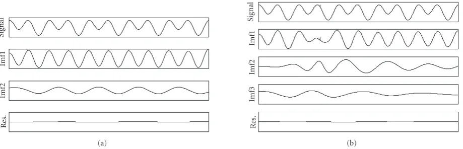
Figure1: (a) The decomposed results of formula (2) and (b) the decomposed results of signal with intermittency signal.

(ii) At any point, the mean value of the envelope defined by the local maxima and the envelope defined by the local minima is zero.

In practice, most of the signals may involve more than one oscillatory mode, that is, the signal has more than one instantaneous frequency at a time locally. Assumed that any data consist of different simple IMFs, EMD is developed to decompose a signal into IMF components and every IMF has a unique local frequency. Given a time series datax(t), it can be decomposed by EMD as follows [1,10].

(1) Identify all the maxima and minima ofx(t).

(2) Generate its upper and lower envelopes,xup(t) and

xlow(t), with cubic spline interpolation.

(3) Compute the local meanm(t)=(xup(t) +xlow(t))/2.

(4) Extract the detail,g(t)=x(t)−m(t). (5) Check whetherg(t) is an IMF or not;

(5.1) if g(t) is an IMF according to the definition of IMF, extract IMF and replacex(t) with the residualr(t)=x(t)−g(t),

(5.2) ifg(t) is not an IMF, further sifting is needed, and replacex(t) withg(t).

(6) repeat steps (1–5) until the residual satisfies some stopping criterion.

The sifting process will be continued until no more IMFs can be extracted. At the end of the decomposition, the signal x(t) is represented as follows:

x(t)= N

j=1

cj(t) +rN(t), (1)

whereNis the number of IMFs,rN(t) is the residue which is a constant, a monotonic, or a function with only maxima and one minima from which no more IMF can be derived, andcjdenotes IMF.

We can apply above EMD procedure to decompose the time series into set of IMFs and a residue. By applying the Hilbert transform to each IMF we can farther analyze the

signal and calculate the instantaneous frequency of each transformed IMF. The whole process is called Hilbert-Huang transform (HHT) [1].

3. EFFECT OF INTERMITTENCY POINT TO EMD

The EMD method has been applied widely in many areas, which shows that it has good effectiveness. Yet straight-forward application of the sifting method may run into difficulties. Especially the original data contain intermittency which will cause mode mixing, that is, the first IMF will contain the information of intermittency signal so that it could not exhibit normal frequency process. Once the first IMF caused mixing phenomenon, the subsequent IMFs will be influenced.

Let us consider the data s(t) given in formula (2). Figure 1(a) shows the decomposed results of s(t) with application of the straightforward EMD, and Figure 1(b) shows the decomposed results ofs(t) including intermittency signal:

s(t)=sin(2p×5t) + 2 cos(2p×10t) + 3. (2)

InFigure 1(b), the first IMF includes the frequency of intermittency signal, that is, mode mixing is caused in the part of intermittency signal. As a result, the subsequent IMFs also contain seriously mixed modes. To explain it more, root mean square error (RMSE), which is expressed as formula (3), is adopted as an evaluation criterion:

RMSE=x(t)−x(t)2/T, (3) wherex(t) denotes decomposed IMF data,x(t) denotes the real signal data, andTis the length of time series.

The RMSE of IMFs can be summarized inTable 1. From Table 1, we can find that errors of IMF components and real value become larger due to intermittent signal. As the mode mixing caused by intermittency is inevitable, it is more worthwhile to explore a method to solve the problem.

4. THE SOLUTION TO INTERMITTENCY PROBLEM

Table1: RMSE of EMD of simulation signal.

IMF1 IMF2 Residue

Normal signal 0.0064 0.0534 0.0720 Abnormal signal 0.3752 1.1341 1.021

Si

gn

al

Im

f1

Im

f2

Im

f3

Im

f4

Re

s.

Figure 2: EMD result of signal after tradition doing wavelet denoising.

considerable interest in the use of wavelet transforms for removing noise from signals. One method has been the use of transform-based threshold, working in three steps:

(i) transform the noisy data into an wavelet domain, and get a group of wavelet coefficients,

(ii) apply soft or hard threshold to the resulting coeffi -cients, thereby suppressing those coefficients smaller than certain amplitude, then obtain a group of estimate coefficients, and

(iii) transform back into the original domain.

Wavelet transform can detect and characterize singulari-ties in signals so that it offers criterion for the classification and identification of signal. Now, there are some studies about comparing wavelet with EMD method [11, 12]. We attempt to adopt the wavelet denoising to eliminate mode mixing, but simulations show that denoising with the traditional wavelet transform can exhibit pseudo-Gibbs phenomena in the neighborhood of discontinuities, which still causes mode mixing. To make our meaning clear, with application of the straightforward wavelet denoising in Haar basis toFigure 1(b), and then using EMD method, we will obtain the components as shown inFigure 2, in which the first two IMF components contain seriously mixed modes. It is evident that the pseudo-Gibbs oscillations caused by wavelet denoising in the vicinity of discontinuities may run into mode mixing. One method to suppress pseudo-Gibbs phenomena is called translation invariant wavelet transform by Coifman and Donoho [13].

4.1. Wavelet threshold denoising based on

translation invariance

In the neighborhood of discontinuities, traditional wavelet denoising can exhibit pseudo-Gibbs phenomena. An

impor-tant observation about the phenomena is that the size of pseudo-Gibbs depends mainly on the location of a discontinuity in the signal. For example, when using the Haar wavelets as basis, a discontinuity located atn/2 will not give pseudo-Gibbs oscillations; a discontinuity nearn/3 will lead to significant pseudo-Gibbs oscillations. The essence reason is the misalignment between the signal data and the basis [14,15].

A possible way to correct the misalignment between the data and the basis is to forcibly shift the data so that the discontinuities change positions, the shifted signal will not exhibit the pseudo-Gibbs phenomena, and after denoising the data can be shifted back. Unfortunately, we do not know the location of the discontinuity. One method solving this situation is optimization: develops a measure of artifacts and minimizes it by a proper choice of the shift, but there is no guarantee that this will always be the case. If the signal has several discontinuities, they may interfere with each other, that is, the best shift for one discontinuity may also be the worst for another discontinuity. Another reasonable approach is called translation invariant algorithm, which is to apply a range of shifts, denoise the shifted data by wavelet threshold and average the several results, then produce a reconstruction subject. Consequently, the shift dependence of wavelet basis is eliminated. This method can effectively suppress the artifacts so that denoised signal is smoother and has better approximation to original signal.

For a signalxt(0≤t < n),Shdenotes the circulant shift byh. TheSh(x)tcan be specifically written as

Sh(x)t=x(t+h) modn. (4) The operator is unitary, and hence invertible:

Sh −1

=S−h. (5)

T represents the process of wavelet transform and denoise based on threshold, the process of eliminating oscillation by translation is shown as follows:

x=S−h

TSh(x)

. (6)

Then apply a range of shifts, so an average over the several results is obtained. For time shifts, we consider a rangeHof shifts and set

x=AVEh∈H

S−h

TSh(x)

, (7)

or in words in order to compare the efficiency with [8], we increased the content. We can draw a conclusion that the efficiency is better than [8] from [13].

The method can be calculated rapidly innlog(n) time [13].

Original signal

−10 0 10

0 100 200 300 400 500 600 700 800 900 1000 (a)

Signal with noise

−20 0 20

0 100 200 300 400 500 600 700 800 900 1000 (b)

Threshold filter

−10 0 10

0 100 200 300 400 500 600 700 800 900 1000 (c)

TA-threshold filter

−10 0 10

0 100 200 300 400 500 600 700 800 900 1000 (d)

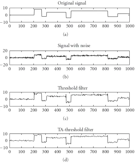
Figure3: Comparison of two denoising methods.

tradition denoising method and the denoising method based on translation invariance algorithm all use Haar as the basis function.

In order to evaluate the effectiveness of the approach, we adopt random square-wave as experimental signal to com-pare traditional threshold algorithm with wavelet transform based on translation invariance algorithm. Both methods decompose the signal with Haar wavelet basis to three layers and use soft threshold denoising which can be defined by [17]

wj,k=

sgnwj,kwj,k−λ

, wj,k≥λ,

0, wj,k< λ,

(8)

where sgn(•) is sign function, one method of choosingλis formula (9):

λ=δ

2 logN, (9)

δ≈Mx/0.6745,Mxrepresents the absolute median estimated on the first scale.

Figure 3shows that comparison between traditional soft threshold and soft threshold based on translation invariance. Here, we average over allncirculant shiftsH = Hn = {h : 0≤h < n}, which are called fully translation-invariant [12]. A benefit of the fully translation-invariant approach is that there are no arbitrary parameters to set: one does not have to decide whether to average over 10 or 20 shifts.

In Figure 3, it displays that denoising method with translation invariance is better than traditional threshold denoising method. The Pseudo-Gibbs phenomenon is elim-inated effectively and the signal curve is smoother.

Table2: Correlation coefficients of two results with original signal.

Traditional threshold TI-threshold

R 0.8271 0.9878

Table3: RMSE of proposed method.

IMF2 IMF3 Residue

RMSE 0.0203 0.0981 0.0954

Using correlation coefficient (R) as an evaluation crite-rion, we compare the two methods with original signal in Table 2. From the data, also we can see that fully translation-invariant threshold is better than traditional threshold when the data includes discontinuity points.

So we can draw a conclusion that TI-threshold wavelet can better solve the problems which the intermittency signal effects on wavelet transform.

4.2. EMD with translation invariance wavelet

transform

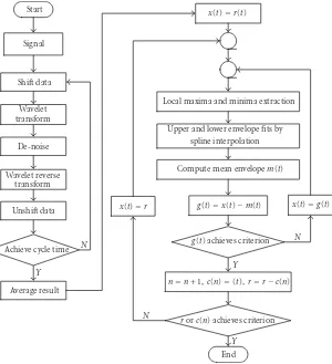
Intermittency signal has the characteristic of sharp variation, so we firstly use wavelet denoising based on translation invariance to pretreat original signal which will eliminate the mode mixing caused by discontinuities. Then, we make use of EMD to extract the IMF components; a set of new modes is obtained. By this way, we can guarantee the validity of EMD method.

The flowchart of the proposed method is shown in Figure 4.

Figure 5 shows the processing result of signal in Figure 1(b)with the proposed method. We can see that the mode mixing phenomenon is eliminated effectively.

Table 3shows the RMSE using proposed method. From the above analysis, it is shown that the denoised signal can be better fitting the real signal by using translation invariance wavelet denoise, which could not blur out important signal features. And the decomposition no longer has mode mixing. Also, the IMFs obtained are closer to real value.

5. APPLICATION TO REAL TEMPERATURE DATA

In order to validate the feasibility of the proposed method, we adopt the data with Zhao [8] to analyze the result.

Start

Signal

Shift data Wavelet transform

De-noise Wavelet reverse

transform Unshift data

Achieve cycle time N Y

Average result

x(t)=r(t)

Local maxima and minima extraction Upper and lower envelope fits by

spline interpolation Compute mean envelopem(t)

x(t)=r g(t)=x(t)−m(t) x(t)=g(t)

N

Y g(t) achieves criterion

n=n+ 1,c(n)=(t),r=r−c(n)

rorc(n) achieves criterion N

Y End

Figure4: The flowchart of the proposed method.

Si

gn

al

Im

f1

Im

f2

Im

f3

Im

f4

Figure5: The EMD result of the proposed method.

result distortion. So, it is necessary to pretreat original data contained intermittency before processing data.

Figure 7displays the results of the application of pro-posed method to the original signal data. The original data pretreat by translation invariance wavelet, the abnormal dis-turbance could be prevented efficiently. Then, decomposing the new dataset by EMD method again, a set of IMFs is obtained, which has a more reasonable physical significance. In this way, we can guarantee the validity of EMD method.

In order to further research the signal features of exceptional temperature, we can remove the residue (res. in Figure 7) and climatic period changing (imf2 inFigure 7), and then restructure the signal.

6. CONCLUSION

In this paper, we analyze the effect of intermittency to EMD method and point out that the signal with intermittency will produce mode mixing phenomenon by directly using EMD approach. Wavelet based on threshold method is an appropriate method for multiscale analysis signal, but it will come into being pseudo-Gibbs phenomena on intermittent points which will affect empirical mode decomposition. So, we adopt translation invariance algorithm to eliminate the artifacts and then proceed to empirical mode decomposition to get IMF components which have genuine physics sense. Theoretical analysis and the given example show that.

(1) The proposed method, which combines empirical mode decomposition and wavelet denoising based on trans-lation invariance algorithm, effectively eliminates the mode mixing caused by intermittency.

Empirical mode decomposition

Si

gn

al

Im

f1

Im

f2

Im

f3

Im

f4

Im

f5

Im

f6

Re

s.

1960 1970 1980 1990

Figure6: Decompose results by straightforward EMD for averaged air temperature.

Si

gn

al

Im

f1

Im

f2

Im

f3

Im

f4

Im

f5

Re

s.

1960 1970 1980 1990

Figure7: EMD results of the method in this paper.

ACKNOWLEDGMENT

The authors would like to thank Professor Zhao Jinping who works in Ocean University of China for providing “Barrow sounding balloon data.”

REFERENCES

[1] N. E. Huang, Z. Shen, S. R. Long, et al., “The empirical mode decomposition and the Hilbert spectrum for nonlinear and non-stationary time series analysis,”Proceedings of the Royal Society of A, vol. 454, no. 1971, pp. 903–995, 1998.

[2] S.-X. Yang, J.-S. Hu, Z.-T. Wu, et al., “The comparison of vibration signal time-frequency analysis between EMD-based HTT and WT method in rotating machinery,”Proceedings of the CESS, vol. 23, no. 6, pp. 102–107, 2003.

[3] Z. K. Peng, P. W. Tse, and F. L. Chu, “An improved Hilbert-Huang transform and its application in vibration signal analysis,”Journal of Sound and Vibration, vol. 286, no. 1-2, pp. 187–205, 2005.

[4] R. Balocchi, D. Menicucci, E. Santarcangelo, et al., “Deriving the respiratory sinus arrhythmia from the heartbeat time series using empirical mode decomposition,”Chaos, Solitons & Fractals, vol. 20, no. 1, pp. 171–177, 2004.

[5] M. C. Ivan and G. B. Richard, “Empirical mode decompo-sition based time-frequency attributes,” inProceedings of the 69th Annual Meeting of the Society of Exploration Geophysicists (SEG ’99), pp. 73–91, Houston, Tex, USA, November 1999. [6] Md. Khademul Islam Molla, M. Sayedur Rahman, A. Sumi,

and P. Banik, “Empirical mode decomposition analysis of climate changes with special reference to rainfall data,”Discrete Dynamics in Nature and Society, vol. 2006, Article ID 45348, 17 pages, 2006.

[7] N. E. Huang, Z. Shen, and S. R. Long, “A new view of nonlinear water waves: the Hilbert spectrum,”Annual Review of Fluid Mechanics, vol. 31, pp. 417–457, 1999.

[8] J. Zhao, “Study on the effects of abnormal events to empirical mode decomposition method and the removal method for abnormal signal,”Journal of Ocean University of Qingdao, vol. 31, no. 6, pp. 805–814, 2001.

[9] H. Li, L. Yang, and D. Huang, “The study of the intermittency test filtering character of Hilbert-Huang transform,” Mathe-matics and Computers in Simulation, vol. 70, no. 1, pp. 22–32, 2005.

[10] G. Rilling, P. Flandrin, and P. Gonc¸alv`es, “On empirical mode decomposition and its algorithms,” inProceedings of 6th IEEE-EURASIP Workshop on Nonlinear Signal and Image Processing (NSIP ’03), Grado, Italy, June 2003.

[11] H. T. Vincent, S.-L. J. Hu, and Z. Hou, “Damage detec-tion using empirical mode decomposidetec-tion method and a comparison with wavelet analysis,” inProceedings of the 2nd International Workshop on Structral Health Monitoring, pp. 891–900, Stanford, Calif, USA, September 1999.

[12] Z.-Q. Gong, M.-W. Zou, X.-Q. Gao, and W.-J. Dong, “On the difference between empirical mode decomposition and wavelet decomposition in the nonlinear time series,”ACTA Physica Sinica, vol. 54, no. 8, pp. 3947–3957, 2005.

[13] R. R. Coifman and D. L. Donoho, “Translation-invariant de-noising,” inWavelets and Statistics, vol. 103 ofLecture Notes in Statistics, Springer, New York, NY, USA, 1994.

[14] S. E. Kelly, “Gibbs phenomenon for wavelets,” Applied and Computational Harmonic Analysis, vol. 3, no. 1, pp. 72–81, 1996.

[15] H.-T. Shim and H. Volkmer, “On the Gibbs phenomenon for wavelet expansions,”Journal of Approximation Theory, vol. 84, no. 1, pp. 74–95, 1996.

[16] B. Tang, C. Yang, S. Tan, and S. Qin, “Denoise based on translation invariance wavelet transform and its applications,” Journal of Chongqing University, vol. 25, no. 3, pp. 1–5, 2002. [17] D. L. Donoho, “De-noising by soft-thresholding,”IEEE