Volume 2006, Article ID 53691, Pages1–6 DOI 10.1155/ASP/2006/53691
Global Motion Model for Stereovision-Based Motion Analysis
Jia Wang,1Zhencheng Hu,2Keiichi Uchimura,2and Hanqing Lu1
1National Laboratory of Pattern Recognition, Institute of Automation, Chinese Academy of Sciences, 95 Zhongguancun East Road,
Beijing 100080, China
2Department of Computer Science, Faculty of Engineering, Kumamoto University, 2-39-1 Kurokami, Kumamoto 860-8555, Japan Received 26 October 2005; Revised 11 January 2006; Accepted 21 January 2006
Recommended for Publication by Dimitrios Tzovaras
An advantage of stereovision-based motion analysis is that the depth information is available, thus motion can be estimated more precisely in 2.5D stereo coordinate system (SCS) constructed by the depth and the image coordinates. In this paper,stereo global motionin SCS, which is induced by 3D camera motion in real-world coordinate system (WCS), is parameterized by a five-parameter global motion model (GMM). Based on such model, global motion can be estimated and identified directly in SCS without knowing the physical parameters about camera motion and camera setup in WCS. The reconstructed global motion field accords with the spatial structure of the scene much better. Experiments on both synthetic data and real-world images illustrate its promising performance.
Copyright © 2006 Hindawi Publishing Corporation. All rights reserved.
1. INTRODUCTION
The advantage of stereovision-based motion analysis is that the depth/disparity information can be computed. Consid-ering the depth information together with the image coordi-nates, motion can be analyzed more precisely in a 2.5D space rather than the traditional 2D image plane. This paper, by expressing the 2.5D space as stereo coordinate system (SCS), addresses the problem of global motion modeling in SCS.
Global motion model (GMM) is commonly used to de-scribe the effect of camera motion (global motion) acting on video image. By GMM, global motion can be distinguished from image motion induced by moving objects (local mo-tion), thus moving objects can be extracted from the image.
In the literature, single-camera-based GMM approaches [1–3], which analyze the camera motion based on 2D image-space shifts [1], cannot describe the global motion accurately when the depth of field is great. By using stereovision, global motion can be estimated more precisely from 2.5D stereo-motion analysis using the depth and image coordinates. The reconstructed global motion field will accord with the spa-tial structure of the scene much better, which makes moving object’s detection much easier.
In this paper, a five-parameter stereo GMM is proposed to parameterize global motion in SCS based on the analy-sis of 3D camera motion. Different from the previous works aiming to recover the physical parameters of camera motion in real-world coordinate system (WCS) [4–8], the presented
model pays more attention to the fast distinguishing of global motion and local motion directly from stereo data. Thus in-stead of estimating the real camera motion in WCS, global motion is estimated and identified directly in SCS with-out knowing the physical camera parameters. The proposed model is provided as a tool for stereo-motion analysis where disparity can be fast calculated. It is very useful for many stereovision-based real-time applications, such as surveil-lance, robot vision, especially of our research on stereovision-based adaptive cruise control (ACC) systems [9].
2. STEREO GLOBAL MOTION MODEL
A typical stereovision system consists of two coplanar cam-eras with the same intrinsic parameters [9]. By projecting a point in WCS (x,y,z) to the stereo left/right ICSs (u,v), the following equation is held:
ul,r= f
x±b/2
z vl,r= f yz , (1)
where f is camera focal andbis baseline distance between the cameras. Then, disparityΔcan be achieved by
Δ=ul−ur= f b
Δ= f bz ,
⎪ ⎪ ⎩z= f b
Δ.
Note that in stereovision, the intrinsic parameters f andb al-ways remain unchanged. Global motion with respect to WCS can be generally referred, as a composition of rotations about x-, y-,z-axes followed by translations along them [10]. To express the stereo GMM in SCS, this paper analyzed the ro-tation and translation separately based on the relationship between WCS and SCS.
In WCS, “rotation aboutx-axis” with angleαcan be de-scribed by ⎡ ⎢ ⎢ ⎣ x y z ⎤ ⎥ ⎥ ⎦= ⎡ ⎢ ⎢ ⎣
1 0 0
0 cosα sinα 0 −sinα cosα
⎤ ⎥ ⎥ ⎦ ⎡ ⎢ ⎢ ⎣ x y z ⎤ ⎥ ⎥
⎦. (4)
Mapping to SCS based on (3), there is
u= u
cosα−sinα·(v/ f),
v= cosα·v+ fsinα cosα−sinα·(v/ f),
Δ= Δ
cosα−sinα·(v/ f).
(5)
In order to deduce a simple expression, we assume that the rotation angleαis small. Sincev/ f is generally smaller than 1, whenαis small, we approximate that
cosα≈1, vsinα
f ≈0. (6) Then (5) can be simplified as
u≈u, v≈v+ fsinα, Δ≈Δ, (7)
which results in aΔ-independent global displacement ofv. Note that such simplification is also permitted by the variety of depths that are being reconstructed.
Similarly, “rotation about y-axis” with angle β is de-scribed by
u= cosβ·u−fsinβ cosβ+ sinβ·u−Δ/2/ f
β→0
≈ u−fsinβ,
v= v
cosβ+ sinβ·u−Δ/2/ f β→0
≈ v,
Δ= Δ
cosβ+ sinβ·u−Δ/2/ f β→0
≈ Δ,
(8)
which results in aΔ-independent global displacement ofu.
Because “rotation aboutz-axis” occurs less frequently than the other motions [2], it will not be considered by the model presented in this paper.
Translations within WCS and their mappings in SCS can be described by
⎡ ⎢ ⎢ ⎣ x y z ⎤ ⎥ ⎥ ⎦= ⎡ ⎢ ⎢ ⎣ x y z ⎤ ⎥ ⎥ ⎦+ ⎡ ⎢ ⎢ ⎣ tx ty tz ⎤ ⎥ ⎥ ⎦=⇒ ⎧ ⎪ ⎪ ⎪ ⎪ ⎪ ⎪ ⎪ ⎪ ⎪ ⎨ ⎪ ⎪ ⎪ ⎪ ⎪ ⎪ ⎪ ⎪ ⎪ ⎩
u= u+Δtx/b 1+Δtz/ f b,
v= v+Δty/b 1+Δtz/ f b,
Δ= Δ
1 +Δtz/ f b,
(10)
which demonstrate that translation alongx/y-axis will bring aΔ-dependent displacement tou/v, respectively, yet transla-tion alongz-axis will change the scale ofu,v, andΔ simulta-neously.
Based on the above analysis, camera’s rotation aboutx-, y-axes and translation alongx-,y-,z-axes are parameterized into such a stereo GMM as
u=u+RY+TXΔ 1 +TZΔ ,
v=v+RX+TYΔ 1 +TZΔ , Δ
= Δ
1 +TZΔ,
(11)
where (RX,RY,TX,TY,TZ) are introduced to describe the rotations and translations by letting RX = f sinα, RY = −f sinβ,TX=tx/b,TY =ty/b,TZ=tz/ f b.
3. PARAMETER ESTIMATION
Corresponding pixel pairs (measured by corner matching or block matching) between successive frames are used to esti-mate the five parameters. Assuming there areNpairs, each pair consists of a pixel k = 1,. . .,N with SCS coordinate (uk,vk,Δk) in the first frame, and its counterpoint (uk,vk,Δk) in the next frame. The five parameters (RX,RY,TX,TY,TZ) are estimated by a least-square method following two steps.
Step 1. Estimating TZ. Based on the third subformula of (11),TZis first estimated by minimizing the following least-square criterion:
TZ=arg min TZ N k=1 Δ
k−1 +TZΔk1 Δk
2
=arg min TZ N k=1 Δ
k+TZΔkΔk−Δk
2.
(a) (b) (c)
(d) (e)
Figure1: Synthetic data involving global motion and local motion. (a) and (b) are the succesive frames where the image intensity denotes disparity. (c) gives the 2D motion field between (a) and (b). (d) is the camera motion compensated image of (a) based on the estimated parameters (RX,RY,TX,TY,TZ)=(6.76,−6.83, 31.17,−28.62, 0.248103). (e) shows the difference between (d) and the actual image (b).
Differentiating (12) with respect toTZand setting the deriva-tive to zero,TZis achieved by
TZ= N k=1
Δ kΔk2
−Nk=1
ΔkΔ k2
N
k=1
Δ kΔk
2 . (13)
Three sums are needed in (13), which can be computed by summing Δof all theN pixel pairs. In addition, in order to avoid the influence of local motion, the above estimat-ing procedure is performed iteratively, which is similar to the method in [2]. In each iteration, every pixel pair is evalu-ated based on the computedTZ by comparing the original Δwith the computedΔusing (11). If the difference exceeds a predefined threshold, corresponding pixel pair will be re-ferred to as local motion pairs and will be discarded. (In our experiments, the threshold is an experiential value which is selected as 0.1.) Then the remaining pairs are used to reesti-mateTZ. Using such method, the influence of pixel pairs that do not follow global motion will be removed gradually and the convergence ofTZwill occur after a very few iterations. (Generally, the convergence will occur with 4 iterations.)
Step 2. Estimating (TX,TY,RX,RY). Based onTZ, we intro-duced an auxiliary variableZk =1 +ΔkTz. Then similar to
the solving ofTZ, the following criteria are minimized:
TX,RY=arg min TX,RY
N
k=1
Zku
k−uk−RY−TXΔK2,
TY,RX=arg min TY,RX
N
k=1
Zkv
k−vk−RX−TYΔk
2 ,
(14)
and (TX,TY,RX,RY) are achieved by
TX= N(
ZuΔ−uΔ) + (u−Zu)Δ N(Δ)2−(Δ)2 ,
RY= (
Zu−u)(Δ)2+ (uΔ−ZuΔ)Δ N(Δ)2−(Δ)2 ,
TY= N(
ZvΔ−vΔ) + (v−Zv)Δ N(Δ)2−(Δ)2 ,
RX= (
Zv−v)(Δ)2+ (vΔ−ZvΔ)Δ N(Δ)2−(Δ)2 ,
(15)
where the subscriptkis omitted for simplification. Note that the estimation of (TX,TY,RX,RY) also follows an iterative scheme, aiming to eliminate the influence of local motion.
4. SIMULATION RESULTS
Figure 1shows the synthetic data where image intensity de-notes disparity. Between Figures 1(a) and 1(b), the cam-era (f = 200,b = 100) undergoes a rotation (α,β) =
(0.01π, 0.01π) and a translation (tx,ty,tz) = (3000,−3000, 5000), while the closest cube undergoes an isolated mo-tion.Figure 1(c)illustrates their correspondence relationship in format of 2D motion vectors, where the local motion is marked by gray vectors. Based on the physical parame-ters of camera motion, the reference GMM parameparame-ters are (RX,RY,TX,TY,TZ) = (6.28,−6.28, 30,−30, 0.250000). Us-ing the two-step iterative estimator, the estimated parame-ters come to be (6.76,−6.83, 31.17,−28.62, 0.228103). In or-der to measure the accuracy of the model and the param-eters, Figure 1(d)shows the predicted image ofFigure 1(a)
after camera motion compensation based on the estimated parameters. A 2D global motion field is also constructed by recomputing the 2D motion vectors using such parameters. The predicted image is compared with the actual image (see
Figure 1(b)), and their difference is shown inFigure 1(e).
Accuracy analysis
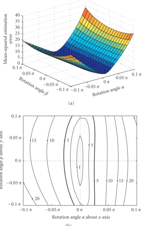
To analyze the accuracy of the stereo GMM quantitatively, we defined a mean-squared estimation error (MSEE) as follows:
MSEE=N1 N k=1
u∗ k −uk
2
+v∗k −v k
2
+Δ∗k −Δ k
2 ,
(16)
where N is the number of the corresponding pairs, (u∗k,vk∗,Δ∗k) is the actual SCS coordinate after camera mo-tion, and (uk,vk,Δk) is the estimated SCS coordinate. Based on the synthetic data in Figure 1, Figure 1 shows the cal-culated MSEE versus physical parameters of camera rota-tion (α,β). It can be seen that when the rotation angles are small, the MSEE is small (MSEE≤ 5 corresponding to re-gions surrounded by thick boundaries inFigure 2(b)) and the stereo GMM can work well. Comparing the two kinds of rotations, MSEE is more sensitive to rotation angleαabout thex-axis. This comes from the fact that many points with largev/ f (v/ f ≈1) are existing at the bottom of the image (as shown inFigure 1(a), where the image size is 400×400, and f = 200), thus the approximation of vsinα/ f ≈ 0 in formula (6) becomes false whenα increases. For trans-lations, the presented GMM can cope with large transla-tions alongx-, y-, andz-axes. We have tested the GMM by
−10000≤tX,tY,tZ ≤10000, and the MSEE remains within 10−6.
5 0
M
ean-squar
0.1π 0.05π
0π −0.05π
−0.1π−0.1π−0.05π
0π 0.05π 0.1π
Ro tatio
n angle
β Rotationangleα
(a) 0.1π
0.05π
0π
−0.05π
−0.1π
Ro
ta
ti
o
n
an
gl
e
β
about
y
-axis
−0.1π −0.05π 0π 0.05π 0.1π Rotation angleαaboutx-axis
20
15 10 5
1 3
5 10 15 20
(b)
Figure2: MSEE versus rotation angle aboutx-,y-axis (α,β): (a) 3D map; (b) contour map.
4.2. Real-world images
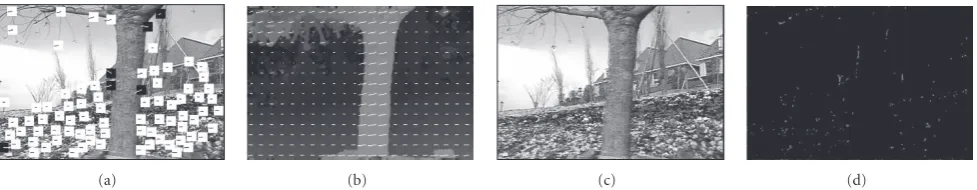
Experiment 1
The testing image is taken from flower garden sequence, which involves an apparent camera motion of translation alongx-axis. Corresponding disparity image is taken from [12] as shown in Figure 3(b). Note that disparity Δ can be computed by various methods with different resolu-tions, it is normalized into 0 ≤ Δ ≤ 1 before estimating
(TX,TY,TZ,RX,RY).Figure 3(a)shows the detected corners
and their 2D motion vectors pointing to the counterpoints in the next frame. Based on such corner pairs, the iterative scheme computes the parameters asTx= −12.434820,Ty=
1.723545,Tz=0.004598,Rx= −0.117074,Ry= −0.099431, where the most apparent global motion is parameterized by
Tx.Figure 3(b)shows the reconstructed 2D global motion
(a) (b) (c) (d)
Figure3: Experimental results onflower gardensequence: (a) original image with the detected corners and their motion vectors; (b) disparity image and reconstructed global motion field using the estimated parameters (Tx = −12.434820, Ty =1.723545, Tz =0.004598, Rx = −0.117074,Ry= −0.099431); (c) camera motion compensated image; (d) difference image between the compensated image and the original image.
(a) (b) (c) (d)
Figure4: Experimental results on a traffic scene: (a) original image with the detected corners and their motion vectors; (b) disparity image and reconstructed global motion field using the estimated parameters (RX,RY,TX,TY,TZ)=(0.05, 0.03, 0.05, 0.71,−0.067826); (c) camera motion compensated image; (d) difference image between the compensated image and the original image.
Figure 3(a), those which do not match are marked by black
color. To our experience, corners which do not follow the global motion are either belonging to the moving objects or the overlapped regions.Figure 3(c)shows the predicted im-age ofFigure 3(a)by camera motion compensation. To re-duce edge distortions, bilinear interpolation has been applied for image compensation by using the image intensities of the four nearest neighboring pixels. The difference image be-tweenFigure 3(c)and the actual imageFigure 3(a)is shown
inFigure 3(d).
Experiment 2
The stereo GMM is also applied to our own stereo sequence of traffic scene (Figure 4), which is obtained by a binocu-lar system [9] mounted on a moving vehicle. Disparity im-age corresponding toFigure 4(a)is shown inFigure 4(b). For estimating the global motion parameters,Figure 4(a)shows the detected corners and their 2D motion vectors pointing to the counterpoints in the previous frame. Based on such cor-ner pairs, the two step estimator computes the parameters as (RX,RY,TX,TY,TZ)=(0.05, 0.03, 0.05, 0.71,−0.067826). Then the reconstructed 2D global motion field is given
in Figure 4(b). Comparing with such field, corners which
match with the field are marked by white color inFigure 4(a), those that do not match are marked by black color. From
Figure 4(a), it can be seen that corners belonging to the
major moving objects are successfully detected, while those
belonging to the slightly moving objects are confused with the background noise.Figure 4(c)shows the predicted im-age ofFigure 4(a)by camera motion compensation. To re-duce edge distortions, bilinear interpolation has been applied for image compensation by using the image intensities of the four nearest neighboring pixels. The difference image be-tweenFigure 4(c)and the actual imageFigure 4(a)is shown
inFigure 4(d).
5. CONCLUSION
Experimental results demonstrate that the proposed stereo GMM works well for stereovision-based camera motion analysis and the motion parameters can be efficiently esti-mated by the two-step iterative estimator. Based on the sented model, global motion can be estimated more pre-cisely according with the spatial structure of the scene, which makes further motion analysis, such as real moving object’s detection, much easier. In addition, the computational sim-plicity of the presented method also makes it suitable for real-time applications such as ACC systems.
ACKNOWLEDGMENT
tion model and global motion compensation,”IEEE Transac-tions on Circuits and Systems for Video Technology, vol. 9, no. 7, pp. 1075–1099, 1999.
[3] G. Qian, R. Chellappa, and Q. Zheng, “Robust Bayesian cam-eras motion estimation using random sampling,” in Interna-tional Conference on Image Processing (ICIP ’04), vol. 2, pp. 1361–1364, Singapore, Republic of Singapore, October 2004. [4] T. S. Huang and S. D. Blostein, “Robust algorithm for motion
estimation based on two sequential stereo image pairs,” in Pro-ceedings of the IEEE Computer Society Conference on Computer Vision and Pattern Recognition (CVPR ’85), pp. 518–523, San Francisco, Calif, USA, June 1985.
[5] G.-S. J. Young and R. Chellappa, “3-D motion estimation us-ing a sequence of noisy stereo images: models, estimation, and uniqueness results,”IEEE Transactions on Pattern Analysis and Machine Intelligence, vol. 12, no. 8, pp. 735–759, 1990. [6] J. Shieh, H. Zhuang, and R. Sudhakar, “Motion esimtation
from a sequence of stereo images: a direct method,” IEEE Transactions on Systems, Man, and Cybernetics, vol. 24, no. 7, pp. 1044–1053, 1994.
[7] H. Hirschmuller, P. R. Innocent, and J. M. Garibaldi, “Fast, unconstrained camera motion estimation from stereo with-out tracking and robust statistics,” inThe 7th International Conference on Control, Automation, Robotics and Vision, vol. 2, pp. 1099–1104, Singapore, Republic of Singapore, December 2002.
[8] Z. Xiang and Y. Genc, “Bootstrapped real-time ego motion es-timation and scene modeling,” inThe 5th International Con-ference on 3-D Digital Imaging and Modeling (3DIM ’05), pp. 514–521, Ottawa, Ontario, Canada, June 2005.
[9] Z. Hu and K. Uchimura, “U-V-disparity: an efficient algo-rithm for stereovision based scene analysis,” inIEEE Intelligent Vehicle Symposium (IV ’05), Las Vegas, Nev, USA, June 2005. [10] A. M. Tekalp,Digital Video Processing, Prentice Hall, Beijing,
China, 1998.
[11] J. Shi and C. Tomasi, “Good features to track,” inProceedings of the IEEE Computer Society Conference on Computer Vision and Pattern Recognition (CVPR ’94), pp. 593–600, Seattle, Wash, USA, June 1994.
[12] S. B. Kang, R. Szeliski, and J. Chai, “Handling occlusions in dense multi-view stereo,” inProceedings of the IEEE Computer Society Conference on Computer Vision and Pattern Recognition (CVPR ’01), vol. 1, pp. 103–110, Kauai, Hawaii, USA, Decem-ber 2001.
Jia Wangreceived his B.E. degree and M.S. degree from Huazhong University of Sci-ence and Technology, China, in 1999 and 2002, respectively. He is currently a Ph.D. Candidate in National Laboratory of Pat-tern Recognition, Institute of Automation, Chinese Academy of Sciences, China. His research interests include video motion analysis, image segmentation, and machine vision applications in ITS.
terests include camera motion analysis,
aug-mented reality, and Machine vision applications in industry and ITS. He is a Member of IEEE, and the Institute of Electronics and Information Communication Engineers of Japan (IEICE).
Keiichi Uchimura received the B.E. and M.E. degrees from Kumamoto University, Kumamoto, Japan, in 1975 and 1977, re-spectively, and the Ph.D. degree from To-hoku University, Miyagi, Japan, in 1987. He is currently a Professor with the De-partment of Computer Science, Kumamoto University. He is engaged in research on in-telligent transportation systems, and com-puter vision. He is a Member of the
Insti-tute of Electronics and Information Communication Engineers of Japan.
Hanqing Luwas born in 1961. He received his B.E. degree and M.S. degree both from Harbin Institute of Technology in 1982 and 1985, respectively. He received his Ph.D de-gree from Huazhong University of Science and Technology in 1992. Since 1992, he has been with the Institute of Automation of Chinese Academy of Sciences, where he is now a Professor. His research interests in-clude image processing, content-based