Damage detection in structures using measured frequency response function data

(1)

VICTORIA UNIVERSITY OF TECHNOLOGY

DAMAGE DETECTION IN STRUCTURES USING

MEASURED FREQUENCY RESPONSE FUNCTION

DATA

by

Abhijit Roy Choudhury

A thesis submitted to the Victoria University of Technology

for the degree of Doctor of Philosophy.

(2)

I would like to express my sincere gratitude to Dr. Jimin He for his untiring

supervision, advice and guidance which have greatly contributed to the

success of this project.

My thanks are also due to Professor Geoffrey Lleonart for his helpful

guidance in writing this thesis. Other members of the staff in the department

of mechanical engineering are also acknowledged for their help at different

stages of this work.

Sincere thanks are also due to all colleagues for their friendly cooperation and

fruitful discussions during the course of the present work.

The author is also thankful to Victoria University of Technology for the

financial support provided over the period in which this work was carried out.

More personally, the author owe most to his parents, wife Amba and sister

Mousumi for their constant support and encouragement, without which this

(3)

ABSTRACT

Modem engineering structures such as offshore oil platforms, transmission

towers, bridges and aircraft frames are regularly monitored and maintained in

order to avert catastrophic failure. Despite our best efforts, sporadic failures,

which may have disastrous consequences in terms of human life and

resources, still occur. It is therefore important to develop techniques which

lead to significant improvements in the reliability of the structures.

A challenging area of structural dynamics research is concerned with the

development and practical implementation of monitoring systems which can

identify and quantify damage as it occurs in a structure. The development of a

number of techniques that contribute to providing means to detect structural

damage is the goal of the work presented in this thesis.

A structural damage detection technique based on constrained minimization

theory, which can both locate and quantify damage in a structure has been

successfully developed. For locating damage only in a structure, a method

which works well in the presence of appreciable measurement noise and

coordinate incompleteness was demonstrated. In addition, a submatrix

procedure was successfully applied to directly identify damaged elements in a

structure instead of the degrees of freedom.

Each of the methods required a finite element model of the undamaged

structure. For applications where such a model was not available, a new

(4)

(5)

NOMENCLATURE

The following list gives the principal use of the symbols in this thesis.

However, a given symbol might be used to denote different quantities under

special situations. The interpretation to be given to a symbol will be clear

from the context in which it is employed.

[A 1 ] - as given in equation (3.3.8)

[A2] - as given in equation (3.3.9)

[AQ] - as explained in equation (2.2.25)

[AMIX] " as defined in equation (3.3.14)

[B] - as defined in equation (5.4.1)

{b} - as defined in equation (5.4.1)

[C] - viscous damping matrix

[D] - as explained in equation (2.2.31)

{D} - vector derived from matrix [D]

{df(Q)} - as defined in equation (2.4.3)

{d(Q)} - as defined in equation (3.2.7) in Chapter 3

d - number of frequency pairs

E - Young's Modulus

e - error function as defined in equation (2.2.9)

e l to e5 - random errors

F - number of unknown non-zero coefficients in the stiffness matrix

{F(Q)} - excitation at frequency Q

[G*] - -[A°]'^[KSQ'][A°]

gi, g2 - constraints in the Lagrange equation

[H] - structural damping matrix in Chapter 1

[H]ij - { A D } J { R ^ } / in Chapter 2

{h} - vector comprising of scaling factors

(6)

[I] - identity matrix

IYY - moment of inertia of cross sectional area about axis Y-Y

I2Z - moment of inertia of cross sectional area about axis Z-Z

[K] - stiffness matrix of the structure

[K]j - j submatrix of stiffness matrix transformed to global coordinate system

[KSQ] - [K]uD ® [K]uD

[AK] - differential stiffness matrix of the structure due to damage

Knn - coefficient of stiffness matrix at rm coefficient location in the matrix.

[kj - diagonal modal stiffness matrix

kr - r modal stiffness

L - Lagrange function

[M] - mass matrix of the strucmre

[AM] - differential mass matrix of the structure due to damage

th

[M]j - j submatrix of mass matrix transformed to global coordinate system

[mj] - diagonal modal mass matrix

m, - r^ modal mass

mm - number of measured modes

m - number of measured coordinates

N - number of degrees of freedom of the system

n^ - number of averages

[P] - contains orthonormalized eigenvectors of ([T] + [S])

[QM] - damage quantification matrix due to change in mass only

[QK] - damage quantification matrix due to change in stiffness matrix

[Q2] - damage quantification matrix due to change in dynamic stiffness

matrix

th

Q2,ij - ij element of matrix [Q2]

{R} - as defined in equation (4.2.12)

{R^}i - ith column of [AD]^[KSQJ] in Chapter 2

[S] - as explained in equation (2.2.32)

s - number of frequency points

(7)

Vll

[TR]

[U]

u

[V]

{ X }

{X}

{Y}

[Y]

[Z(^)]

Z(Q)D,ij

{ZUD(")}J

[ZSQ]

[AZ(Q)]

[a(Q)]

{aD(Q)}k

{aD(f)(Q)}k

{auD(^)}k

{Aa(Q)}k

akk(Q)

{P(^)}

{ S } K

Yxy'(^)

[<!)]

TlK

- transformation matrix

- as defined in equation (2.2.10)

- number of unmeasured coordinates

• diagonal matrix whose diagonal elements are the eigenvalues of

([T] + [S])

- as defined equation (2.2.20) in Chapter 2

- as defined equation (5.4.1) in Chapter 3

- dynamic stiffness matrix of the structure

- ij^ element of dynamic stiffness matrix of damaged structure at

frequency Q

- j ' \ o w o f [Z(Q)]uD

- 0.25 [ZJuD <8) [Z]uD

- differential dynamic stiffness matrix of the structure due to damage

at frequency Q

- receptance matrix at frequency Q

th

- k column of the RFRF matrix of the damaged structure at

frequency Q

- k column of the filtered RFRF matrix of the damaged structure at

frequency Q

til

- k column of the RFRF matrix of the undamaged structure at

frequency Q.

th

- k column of the differential RFRF matrix between damaged and

undamaged structure at frequency Q

- kk element of receptance matrix at frequency Q

- damage location vector

- delta vector whose k element is unity

- coherence at frequency Q

- mass normalised mode shapes

th

(8)

X,\i - Lagrange multipliers

[\\f] - eigenvector matrix

[kf\ - diagonal matrix whose diagonal elements are the eigenvalues

>uk - k eigenvalue

BQ* - defined in equation (3.2.20) in Chapter 3

Q - frequency of the system

th

COK - k natural frequency

Operators and symbols

S - summation

{ }^» [ ]^ " transpose

0 - matrix element by element operation

[ ]-l - standard inverse

[ ]+ - pseudo inverse

II II - matrix norm

[ ]i5 - represents damaged structure

[ luD " represents undamaged structure

{*"} - superscript m refers t o measured coordinate

{"} - superscript u refers to unmeasured coordinate

Abbreviations

CDLV - cumulative damage location vector

CMDQ - constrained minimization damage quantification

COMAC - coordinate modal assurance criterion

D. E - dynamic expansion

DLP - damage location plot

DLV - damage location vector

DOF -degree of freedom

(9)

IX

FEM - finite element model

FRF - frequency response function

IRS - improved reduced system

MAC - modal assurance criterion

MDOF -multiple degree of freedom

MRPT - minimum rank perturbation technique

PMAC - partial modal assurance criterion

RFRF - receptance frequency response fiinction

SDOF - single degree of freedom

SEREP - system equivalent reduction expansion process

(10)

Figure Title Page

2.1 Graph showing variation of normalized random error as a 58 function of coherence and number of averages

2.2 Graph of normalized random error and number of averages 58

2.3 Flowchart of program for computer implementation of 59 CMDQ method

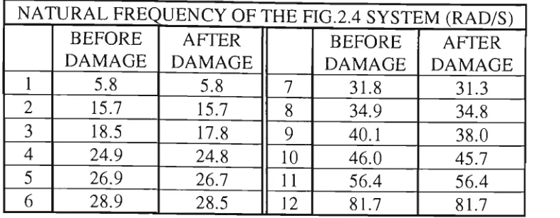
2.4 A 12 DOF mass-spring system (Model 2.1) 60

2.5 An 8 DOF mass-spring system (Model 2.2) 60

2.6 A 20 member plane truss structure (Model 2.3) 61

2.7 Actual [AK] for model 2.1 62

2.8 Calculated [AK] using CMDQ method for pure data in 62 model 2.1 (29 valid eigenvalues; 3, 12, 14 rad/s)

2.12 Calculated [AK] using CMDQ method for pure data in 63 model 2.1 (25 valid eigenvalues; 8, 10, 11, 13 rad/s)

(11)

XI

model 2.1 (29 valid eigenvalues; 8, 10, 11, 13, 15.4rad/s)

2.14 Calculated [AK] using CMDQ method for 2% noisy data in 63 model 2.1 (29 valid eigenvalues; 3, 12, 14 rad/s)

2.15 Calculated [AK] using CMDQ method for 2% noisy data in 64 model 2.1 (29 valid eigenvalues; 3, 12, 14, 13 rad/s)

2.16 Calculated [AK] using CMDQ method for 2% noisy data in 64 model 2.1 (29 valid eigenvalues; 3, 12, 14, 13, 16 rad/s)

2.17 Calculated [AK] using CMDQ method, 2% noisy data in 64 model 2.1 (29 valid eigenvalues; 3, 12, 14, 13, 16, 9 rad/s)

2.18 Calculated [AK] using CMDQ, noise filtering for 2% noisy 64 data in model 2.1 ( 3, 12, 14, 13, 16 rad/s)

2.20 Calculated [AK] using CMDQ method for pure data in 65 model 2.2 (16 valid eigenvalues; 8, 14 rad/s)

2.22 RFRF for model 2.3 before and after damage 66

2.24 Calculated [AK] using CMDQ method for pure data in 66 model 2.3 (12, 19, 25, 43 rad/s)

2.25 Calculated [AK] using CMDQ method for 2% noisy data in 67 model 2.3 ( 12, 19, 25, 43 rad/s)

2.26 Calculated [AK] using CMDQ method for 2% noisy data in 67 model 2.3 (12, 19, 25, 37, 43 rad/s)

(12)

3.1 A 5 DOF mass-spring system 110

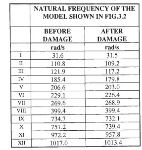
3.2 A 12 DOF mass-spring system (Model 3.2) 110

3.3 A truss structure (Model 3.3) 111

3.4A 3-D DLP using D.E A (Case 1/ Subcase 1 in section 3.4) 112

3.4B 3-D DLP using D.E B (Case 1/ Subcase 1 in section 3.4) 112

3.4C 3-D DLP using D.E C (Case 1/ Subcase 1 in section 3.4) 112

3.4D 3-D DLP using FRF mix (Case 1/ Subcase 1 in section 3.4) 112

3.4E 3-D DLP using SEREP 1 (Case 1/ Subcase 1 in section 3.4) 113

3.4F 3-D DLP using SEREP2 (Case 1/ Subcase 1 in section 3.4) 113

3.4G 3-D DLP using SEREP3 (Case 1/ Subcase 1 in section 3.4) 113

3.4H 3-D DLP using SEREP4 (Case 1/ Subcase 1 in section 3.4) 113

3.5A 3-D DLP using D.E A (Case 1/Subcase 2 in section 3.4) 114

3.5B 3-D DLP using D.E B (Case!/Subcase 2 in section 3.4) 114

3.5D 3-D DLP using FRF mix (Case!/Subcase 2 in section 3.4) 114

3.5E 3-D DLP using SEREPl (Case 1/ Subcase 2 in section 3.4) 115

3.5F 3-D DLP using SEREP2 (Case 1/ Subcase 2 in section 3.4) 115

3.5G 3-D DLP using SEREP3 (Case 1/ Subcase 2 in section 3.4) 115

3.5H 3-D DLP using SEREP4 (Case 1/ Subcase 2 in section 3.4) 115

(13)

X l l l

3.6B/1 CDLV using D.E B (Case 11/ Subcase 1 in section 3.4) 116

3.6C/1 CDLV using D.E B (Case 11/ Subcase I in section 3.4) 117

3.6D 3-D DLP using FRF mix (Case Il/Subcase 1 in section 3.4) 117

3.6D/1 CDLV using FRF mix (Case 11/ Subcase 1 in section 3.4) 117

3.7A/1 CDLV using D.E A (Case 11/ Subcase 2 in section 3.4) 118

3.7B/1 CDLV using D.E B (Case 11/ Subcase 2 in section 3.4) 118

3.7C/1 CDLV using D.E C (Case 11/ Subcase 2 in section 3.4) 119

3.7D 3-D DLP using FRF mix (Case Il/Subcase 2 in section 3.4) 119

3.7D/1 CDLV using FRF mix (Case 11/ Subcase 2 in section 3.4) 119

3.8A 3-D DLP using D.E A (case 1/ subcase I; fig.3.3 model) 120

3.8B 3-D DLP using D.E A (case 1/ subcase II; fig.3.3 model) 120

3.8C 3-D DLP using D.E A (case 1/ subcase III; fig.3.3 model) 120

3.9A 3-D DLP using D.E A (case 2/ subcase I; fig.3.3 model) 121

3.9B 3-D DLP using D.E A (case 2/ subcase II; fig.3.3 model) 121

3.9C 3-D DLP using D.E A (case 2/ subcase III; fig.3.3 model) 121

(14)

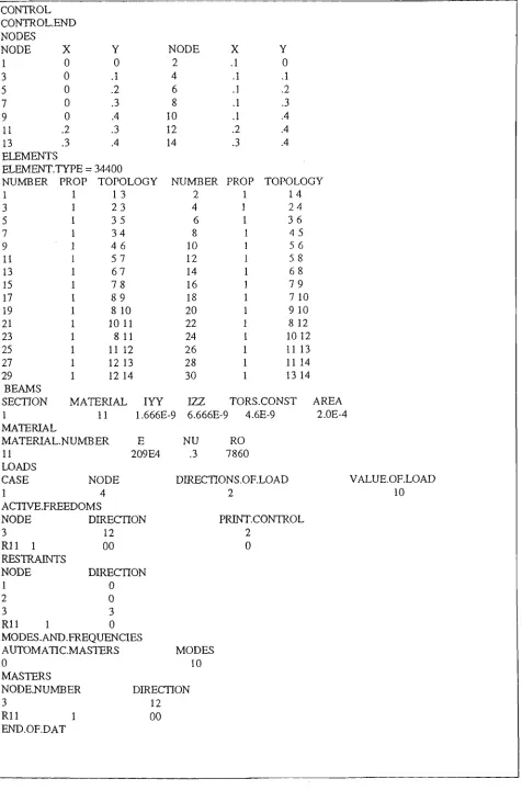
4.3 A cantilever truss structure 144

4.4 Scaling factor due to damage in model 3.2 145

4.5 Identified scaling factor (Approach 1; 2 frequency points, 145 no noise)

4.6 Identified scaling factor (Approach 1; 4 frequency points, 146 no noise)

4.7 Identified scaling factor (Approach 2; no noise) 146

4.8 Identified scaling factor (Approach 1; 4% noise) 147

4.9 Identified scaling factor (Approach 2; 4% noise) 147

4.10 Identified scaling factor (Approach 2 and DLP; 4% noise) 148

4.11 Identified scaling factor (Approach 2, incomplete 148 measurement; 4% noise)

4.12 Identified scaling factor (Approach 2 and DLP; 149 measurement available; 4% noise)

4.13 Identified scaling factor (Approach 2 and DLP; 149 interpolated data; 4% noise)

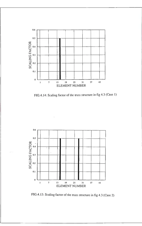
4.14 Scaling factor of the truss structure in fig. 4.3 (Case 1) 150

4.15 Scaling factor of the truss structure in fig. 4.3 (Case 2) 150

4.16 3-D DLP for case 1 damage in fig. 4.3 model 151

4.17 Identified scaling factor for the truss structure in fig.4.3 151 (Casel)

(15)

XV

4.19 Identified scaling factor for the truss structure in fig.4.3 152

(Case2)

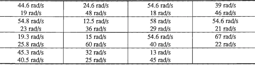
5.2 A continous beam and its lumped mass model 179

5.3 [AK] for the 12 DOF mass-spring system in fig. 3.2 180 5.4 Calculated [AK] for the 12 DOF mass-spring system in fig. 180

3.2 (using Method I in section 5.5.1)

5.5 Calculated [AK] for the 12 DOF mass-spring system in fig. 181 3.2 (using Method II in section 5.5.2)

5.6 Identified scaling factor for fig. 3.2 system (Method III in 181 section 5.5.3; 4% noise)

5.7 Calculated [AK] for fig. 3.2 system (using Method II, 182 frequency points different from case represented in fig.5.5)

5.8 Identified scaling factor for fig. 3.2 system (Method III in 182 section 5.5.3; 4% noise, frequency different from case

represented in fig. 5.6)

5.9 Calculated [AK] for fig. 3.2 system (using Method II, 4% 183 noise, incomplete coordinates measured)

5.10 Identified scaling factor for fig. 3.2 system (Method III in 183 section 5.5.3; 4% noise, incomplete coordinates measured)

5.11 Calculated [AK] for fig. 3.2 system (using Method II, 4% 184 noise, incomplete coordinates interpolated)

5.12 Identified scaling factor for fig. 3.2 system (Method III in 184 section 5.5.3; 4% noise, incomplete coordinates

interpolated)

6.1 A beam structure 223

(16)

6.3a Location on the beam where measurements were taken 225

6.3b Location on the grid where measurements were taken 225

6.4 Schematic diagram of the measurement set-up 226

6.5 Photograph of the experimental rig 226

6.6 a n 1 i(Q) for the beam from measurement and FE model 227

6.7 Coherence of RFRF ( a n ii(Q)) for the undamaged beam 228

6.8 oty 7(Q) for the grid from measurement and FE model 229

6.9 Frequency response of different forms of attachment 229

6.10 aii,i i(^) for the beam before and after damage 230

6.11a 3-D DLP for the beam 231

6.11b CDLV for the beam 231

6.12 a7,7(^) for the grid before and after damage 232

6.13a 3-D DLP for the grid structure 233

6.13b CDLV for the grid structure 233

6.14A a i 1,11(^) for the beam (regenerated, before and after 234 damage) for case A

6.14B a i 1,11(^) for the beam (regenerated, before and after 234 damage) for case B

6.14C tt] 11 i(Q) for the beam (regenerated, before and after 235 damage) for case C

6.15A ai 11 i(Q) for the beam (regenerated, before and after 235 damage) using scaling factor . 15

(17)

damage) using scaling factor .17

XVll

6.15C ai 11 i(Q) for the beam (regenerated, before and after damage) using scaling factor .26

236

6.16A a-jjiQ) for the grid (regenerated, before and after damage for case A

6.16B ay 7(Q) for the grid (regenerated, before and after damage for case B

6.16C ay 7(Q) for the grid (regenerated, before and after damage for case C

6.16D a7 7(Q) for the grid (regenerated, before and after damage for case D

6.17A ajj(Cl) for the grid (regenerated, before and after damage using scaling factor .38

6.17B a7 7(Q) for the grid (regenerated, before and after damage using scaling factor ..24

6.17C a7 7(Q) for the grid (regenerated, before and after damage using scaling factor .37

6.17D a7 7(Q) for the grid (regenerated, before and after damage using scaling factor .34

237

238

239

240

6.18 ot7 7(Q) for the grid (undamaged and after both damages) 241

6.19a 3-D DLP for the grid for both damages 242

(18)

TITLE i

ABSTRACT ii

ACKNOWLEDGEMENTS iv

NOMENCLATURE v

LIST OF FIGURES x

TABLE OF CONTENTS xviii

1. INTRODUCTION 1

1.1 Damage location using measured receptance FRF data 1

1.2 System models 4

1.3 Review of previous work 10

1.4 Assumptions of this study 16

1.4 Scope of present work 17

2. DETERMINATION OF STRUCTURAL DAMAGE EXTENT

USING CONSTIiAINED MINIMIZATION THEORY 20

2.1 Introduction 20

2.2 Constrained minimization damage quantification (CMDQ) method 23

2.3 Discussion 34

(19)

XIX

2.3.2 Determining the number of frequency points 37

2.3.3 Simultaneous mass and stiffness changes due to damage 38

2.4 Noise filtering algorithm for proposed method 40

2.5 Results of numerical analysis 43

2.6 Summarising remarks 51

3. DAMAGE LOCATION IN A STRUCTURE USING MEASURED

FRF DATA 68

3.1 Introduction 68

3.2 Theory of damage location using FRF data 71

3.3 Compatibility of measured and analytical data 77

3.3.1 Reduction Techniques 78

3.3.2 Expansion Techniques 81

3.4 Results of numerical simulations 89

3.5 Analysis of numerical results 99

4. SUBMATRIX APPROACH FOR DETERMINING DAMAGE

EXTENT IN A STRUCTURE 122

4.1 Introduction 122

4.2 Theory of determining damage extent using submatrix approach 124

4.3 Discussions 131

(20)

5. USING SPATIAL MODEL TO DETERMINE DAMAGE

EXTENT 153

5.2 Review of previous works for spatial model derivation 154

5.3 Theory to generate spatial model 157

5.4 Discussion 163

5.5 Application of the method for determining damage extent 166

5.5.1 Method I (Direct Method) 166

5.5.2 Method II (Indirect Method) 167

5.5.3 Method III (Using Submatrix Approach) 168

5.6 Results of numerical case studies 169

6. EXPERIMENTAL CASE STUDY 185

6.2 The test structures 186

6.3 Measurement equipment 186

6.4 Calibration of the measurement equipment 188

6.5 FE modelling of undamaged structure 189

(21)

XXI

6.5.2 Cross stiffened grid structure 190

6.6 Test structure preparation for measurement 190

6.6.1 Support Condition 190

6.6.2 Type of Excitation 191

6.6.3 Attachment and location of transducer 192

6.7 Introduction of damage in the structure 193

6.8 Execution of the measurement 193

6.9 Damage location 194

6.10 Discussion of location results 197

6.11 Determination of damage severity 198

6.12 Discussion of damage severity results 207

6.13 Location of multiple damage 211

7. CONCLUSION AND SUGGESTIONS FOR FUTURE

RESEARCH 243

7.1 General conclusion 243

7.2 New contributions of present research 245

7.3 Suggestions for further work 246

REFERENCES 248

(22)

APPENDIX B 265

APPENDIX C 269

APPENDIX D 272

(23)

CHAPTER 1 INTRODUCTION

With the progress of materials science, new materials have been introduced

which have made it possible to build large and complicated structures with

reduced weight. However, due to the large size and complexity of such

structures and the possible catastrophic effect associated with their failure, it is

imperative to develop a technique which is able to locate, and determine the

extent, of structural damage as it develops in a structure. Advancement in recent

years in the capability of modem electronic instrumentation for signal

processing have resulted in the development of superior instruments for

monitoring the condition of machines. From experience gained in the

machinery health monitoring field, it is expected that the vibration signature of

a structure should provide adequate and useful information to detect possible

structural damage.

1.1 DAMAGE LOCATION/QUANTIFICATION USING MEASURED RECEPTANCE FRF (RFRF) DATA

As a result of the consequences associated with the failure of some present day

structures, in terms of both human life and resources, a lot of effort has been

directed towards developing a suitable technique for detecting damage in

structures. Most of the work in structural damage detection uses the general

framework of model refinement or model updatings where the analytical spatial

(24)

experimental modal model of the damaged structure (natural frequencies and

mode shapes) have been used together to determine damage location and its

extent. In these approaches it is assumed that the analytical model of the

undamaged structure truly represents the structure within certain frequency

ranges of interest.

Although the system identification technique is a promising method in

structural damage detection, use of modal parameters introduces some

disadvantages and limitations into these methods. The experimental modal

parameters of a system by themselves usually present a limited amount of data.

This is because these modal parameters are restricted only to natural frequencies

and mode shapes of the system within the measured frequency range. For most

practical applications the measured frequency range contains only a limited

number of natural frequencies. In addition, if the modal parameters available are

not severely affected by damage, then it would be difficult to detect damage by

applying existing methods using modal parameters.

To generate a true analytical model of a structure, it is required to discretize it

into a large number of degrees of freedom (DOFs). If the number of DOFs is N,

then the complete modal model of the structure should have information about

all N natural frequencies and their corresponding mode shapes. However, the

experimental modal model obtained for a structure is incomplete, as it becomes

difficult to measure over a wide frequency band if the value of N is large. In

addition, it is impractical to measure as many coordinates as an analytical

model has. A few of the earlier methods which required a complete

(25)

Chapter 1: Introduction

unsatisfactorily when working in practical situation. In addition, use of modal

parameters for detecting damage involves the extraction of them from

measured frequency response function (FRF) data by an analysis method called

experimental modal analysis, which may introduce additional computational

burden and errors.

However, if a suitable technique can be developed which makes use of the

analytical spatial model and the experimental response model (FRF data)

instead of the modal model, then it is possible to eliminate most of the

limitations and disadvantages associated with using the modal model.

Therefore, in contrast to the existing structural damage detection methods based

on system identification using the.

Spatial Model Of The Undamaged Structure + Modal Model Of The

Damaged Structure,

the method proposed in this work will use the.

Spatial Model Of The Undamaged Structure + Response Model Of The

Damaged Structure

to locate and quantify damage in the structure. These models are described in

the next section.

However, two problems which confront any structural damage detection

(26)

• effect of noise - in spite of all the technological advances in electronic

instrumentation, it is hard to envisage a condition where no noise of any type

has contaminated the measured vibration data. When using FRF data

directly, it is possible to judiciously select frequency points with a high

signal to noise ratio but it is unlikely that the noise effect will be zero.

• effect of DOF incompleteness - when developing a finite element model of a

structure, it is possible to use a large number of DOFs to discretize it in order

to better resemble the structure. However, while taking measurements of the

structure, it is not possible to measure at all the DOFs corresponding to the

finite element model (FEM) of the structure. One way to tackle this problem

of DOF incompatibility is either to expand the measured DOFs to equal to

FE model DOFs or to reduce the FE model in accordance with the measured

DOFs. However, both the expansion and reduction methods introduce

inaccuracy into the data.

These two problems will be addressed in the context of using FRF data to locate

and determine the extent of structural damage.

1.2 SYSTEM MODELS

The dynamic properties of a system, analytically or experimentally derived, can

be represented in the following model formats: spatial model, modal model and

response model. For the application of damage detection, either the

experimental modal model or the experimental response model of the damaged

(27)

Structure to detect the possible location and extent of damage. These three

models used to describe the dynamic properties of the system are defined

below.

(1) Spatial Model

When a given structure is discretized analytically, spatially distributed

properties, such as the mass, stiffness and damping, are assigned to each of the

N DOFs. These properties are presented in matrix form as given below:

[M]NXN " mass matrix whose diagonal terms define the inertia force assigned

to each DOF when they experience an acceleration and whose off-diagonal

terms contain inertia coupling information.

[K]NXN ~ stiffness matrix whose diagonal terms define the inherent restoring

forces due to relative displacement at each DOF and the off-diagonal terms

express the static coupling between DOFs.

[C]NXN or [H]NXN " viscous and structural damping matrices respectively. In

cases where the dissipative forces are negligible, they are often neglected.

If a spatial model has N co-ordinates, then it is expected to have N modes.

However, if it is reduced by one of the reduction methods to be discussed in

Chapter 3, to 'm' co-ordinates (m < N), it will contain information on 'm'

(28)

Spatial models are also referred to as "Time Models", since equations of motion

formulated by using spatial properties contain the response motions of system

as fiinctions of time.

(2^ Modal Model

Dynamic properties of a system are also often described in terms of natural

frequencies, modal damping factors and associated mode shapes. A

mathematical model comprising these data is called a modal model.

Mathematically, the mode shapes are represented as vectors in which each

element represents a deflection of one DOF relative to the other (N-1) DOFs in

the model. The mode shapes (or eigenvectors) can be grouped together in the,

so called Modal Matrix which is represented by [^]Nxm- This is a square or

rectangular matrix containing information about N co-ordinates and m modes.

The eigenvalues related to system natural frequencies can be grouped together

forming a diagonal matrix represented by [XrJmxm- Generally, both matrices are

th

complex. The k eigenvalue is given here as X^ and the corresponding mode

shape as {^jk- The diagonal matrix corresponding to system natural

frequencies and the modal matrix is presented next:

(29)

M N . . =

af+ibf

a2'+ib;

< +

'K

(1.2)

The k^ eigenvalue contains information related to the k^ natural frequency (co^)

and modal damping (ri^). The k^ mode shape {\)/}i^ is represented by a real part

and an imaginary part.

Since the mode shapes represent relative amplitudes at the DOFs, rather than

absolute deflections of the structure, the elements of each mode shape can be

scaled arbitrarily. For instance, they can be scaled in such a way that the largest

element becomes unity for graphical visualisation purposes. On other occasions,

mode shapes may be required to be uniquely defined. This can be achieved by

making use of the concept of modal mass and modal stiffness. Due to the

orthogonality theory of a multi-degree-of-freedom system, the following

relationships hold (if m < N):

Nxm

(1.3)

(1.4)

With [K] assumed as a complex stiffiiess matrix, equations (1.3) and (1.4) gives

the diagonal modal mass and modal stiffiiess matrices whose elements are

k /

interrelated as X^ = y = coJ(l-i-iT]J. The mode shapes of the system can be

(30)

1-0.5

W-Mk]" (1.5)

where [(j)] is called the mass normalized mode shape. This will result in a new

set of orthogonality equations given below as:

['t'lLjM],,J(|)],.„=[I]_ (1.6)

[ C N M » . H W . . „ = [ ^ , L „ (1.7)

These mass normalized mode shapes can be experimentally obtained from a

modal analysis process, as illustrated by Ewins [1].

(3) Response Model

A linear, time invariant dynamic system, when subjected to a certain input, will

generate a definite output. The basic system equation is:

OUTPUT = SYSTEM CHARACTERISTICS x INPUT (1.8)

It can be seen that the output response is related to the input via its dynamic

characteristics. Using the same system equation for any linear system excited by

harmonic excitation, the input/output relationship in the frequency domain at

frequency Q can be written as:

{X(Q)} = [a(Q)]{F(Q)} (1.9)

(31)

Chapter I: Introduction

where [a(Q)] and [Z(Q)] are related by the following relationship.

[Z(Q)] = [a(Q)]-^ (1.11)

[a(Q)] is called the receptance frequency response function matrix of the

system. The receptance FRF matrix [a(Q)] will become the Mobility matrix or

Inertance matrix if the response measured is velocity or acceleration. In these

matrices each element is a complex ratio (response/force) called the FRF which

covers a certain frequency range. In addition, there exists three other formats for

FRF data, these being the inverse of receptance, mobility and inertance. They

are generally known as 'dynamic stiffiiess', 'mechanical impedance' and

'apparent mass' respectively. The response model is then expressed as an FRF

matrix which may be derived either analytically or experimentally.

It is important to comprehend different practical implications if measuring

[a(Q)] or [Z(Q)]. Consider an element aij(Q)in matrix [a(Q)]. It represents the

amplitude and relative phase of a harmonic displacement at DOF 'i' due to a

harmonic force applied at DOF ' j ' (no other external forces are applied to the

system). However, Zij(Q) represents the amplitude and relative phase of a

harmonic force applied to DOF 'i' due to a unit displacement at DOF ' j ' (when

no other displacement exists in the system).

For a SDOF system it is easy to measure or calculate either a(Q) or Z(Q). For a

MDOF system, it is physically impossible to measure [Z(Q)] since it is

impossible to ensure displacement response only at one DOF while

(32)

Elements in a particular column of matrix [a(Q)] can be measured by changing

the point of response while force location is the same. According to the

reciprocity principle, matrix [a(Q)] is symmetric. Therefore, measuring one

column is equivalent to measuring one row, although the mechanism of

measurement is different.

To summarize, the Response model of a dynamic system can be described by

the FRF matrix whose elements can be either measured or analytically

calculated or sometimes, a mixture of both.

1.3 REVIEW OF PREVIOUS WORKS

Using vibration test data to locate structural damage has been attempted by

many researchers in recent years. A brief review is given here. More details are

given in later chapters where some specific techniques are studied.

Most of the prior work in structural damage detection is based on the general

framework of FEM refinement (System Identification) techniques. The need for

FEM refinement of a structure arose because of the deviation that occurred

between the modal properties predicted by the Finite Element Model and that

measured. To reduce this deviation, the technique of FEM refinement was used

where measurement data of a structure was used to tune or correct the FEM of

the structure. The tuned or correlated FEM is expected to represent the actual

structure more accurately. Unlike model refinement, where the deviation is

(33)

Chapter 1: Introduction 11

attributed to the damage in the structure. This explains the reason behind the

application of the FEM refinement algorithm to damage location problems.

The FEM refinement algorithms which may be used for structural damage

detection may be broadly divided into three categories: optimal matrix

updating, eigenstructure assignment and sensitivity analysis. Among these

categories, perhaps the most widely used is optimal matrix updating. Early

work in this area included that of Rodden [3] who used vibration test data to

determine the structural influence coefficients of a structure. The problem of

finding a matrix that satisfies a set of measurements as well as symmetry and

positive definiteness was addressed by Brock [4]. Berman and Flannely [5]

discussed the calculation of system matrices when the number of DOFs and the

number of measured modes do not coincide.

Several optimal matrix update algorithms are based on the problem formulation

set forth by Baruch and Bar Itzhack [6]. In their work, a closed form solution

was developed for the minimal Frobenius norm matrix adjustment to the

structural stiffness matrix incorporating measured natural frequencies and mode

shapes. Berman and Nagy [7] adopted a similar formulation but included

approaches to improve both the mass and stiffiiess matrices. In their work, the

refined stiffiiess (mass) takes a form in which the original physical connectivity

of the system is destroyed. In separate publications Kabe [8] and Smith and

Beattie [9] suggested algorithms which preserved the original connectivity of

(34)

The Kabe [8] algorithm utilised a percentage change in the stiffness value cost

function and preserved the coimectivity of the original structure. Assuming that

the accurately measured mode shapes of the damaged structure were available

at every finite element DOFs of the structure, Smith and Hendricks [9]

investigated the extent of structural damage. However, in this case the stiffness

matrix coefficients corresponding to undamaged members were significantly

affected, making the detection uncertain. Although the minimization of the

matrix norm of the stiffness difference before and after damage might be a

promising mathematical method, the success of such a method depends heavily

on the introduction of adequate and necessary physical constraints.

The control-based eigenstructure assignment technique determines the

pseudo-control that would be required to produce the measured modal properties with

the initial Finite Element model. The pseudo-control is then translated into

matrix adjustments applied to the initial FEM. Among the approaches described

by Inman and Minas [10], the first approach corrected the stiffness matrix using

information about the eigenparameters. The symmetry in the resultant model

was enforced by using an unconstrained numerical non-linear optimization

approach. The second approach based upon eigenvalue information used a state

space formulation to find the errors due to damage. Zimmerman [11] used a

symmetry preserving eigenstructure assignment theorem where the information

regarding eigenparameters of the damaged structure was incorporated in the

spatial model of the undamaged structure. This algorithm used the solution of a

generalized algebraic Riccati equation whose dimension was defined solely by

(35)

Sensitivity analysis for damage detection makes use of the derivatives of modal

parameters with respect to physical design variables. The derivatives are then

used to update the physical parameters. These algorithms result in updated

models consistent within the original finite element programme framework.

Hajela and Soeiro [12] and Soeiro [13] made direct application of non-linear

optimization to the damage detection problem. Among other works reported

that uses sensitivity analysis, Jung and Ewins [14] described the application of

an inverse eigensensitivity method for model updating using arbitrarily chosen

macro elements to a simple frame. Although the method has been shown to be

reasonably insensitive to noise, the number of eigensensitivity vectors (derived

from eigenvectors) required for the method to succeed might become

prohibitively large for complicated structures.

In addition to the methods discussed above, Liu and Yao [15] considered the

development of the probabilistic methodology for the prediction of multiple

crack distribution in a structure of beam elements. The probabilistic measure of

crack distribution could then be used for probabilistic diagnosis of crack

location and extent. Several other authors have also shown that crack locations

could be identified by using the concept of fracture mechanics along with

information about change in natural frequencies due to damage. Among them

was Gudmundson [16] who used saw cuts to simulate open cracks and the

experimental results obtained by him from vibration measurements agreed

remarkably well with the predictions from the open crack mathematical model

(36)

Chondros and Dimarogonas [17] also created actual fatigue cracks in welded

joints and established a simple relationship between the crack depth and its

flexibility using concepts of fracture mechanics. However, although it is

relatively easy to create an open crack mathematical model of a simple beam, it

may be difficult to apply it to real life structures. Among other researchers in

this area who tried to analyse the change in natural frequencies due to damage

by using fracture mechanics, a notable contribution has been made by Ju [18]

who used the concept of structural modal frequency and concluded that it would

change with the presence of fracture damages in the structure. In his approach,

Ju used fracture mechanics to define a damage characteristic and assumed that

the changes in modal frequencies were functions of damage characteristics.

A different approach to identifying system matrices was suggested by Lim [19]

which was described as a 'submatrix' approach. Instead of working with

individual coefficients in the stiffiiess matrix affected by damage, the submatrix

approach focused on individual blocks or submatrices which often coincided

with individual physical components in the structure. Heam and Testa [20]

studied the dependence of natural frequencies and modal damping coefficients

on structural deterioration and tried to establish the magnitude of change in

natural frequencies as a function of location and severity of deterioration.

Adams et al. [21] used the decrease in natural frequencies and increase in

damping to detect cracks in fibre reinforced plastics. They developed a

theoretical model to detect the damage location but the model seems to be valid

only for simple beam structures. Adams and Cawley [22] employed sensitivity

(37)

Chapter I: Introduction 15

on the finite element analysis method, but this method appears to be

computationally intensive. Yuen [23] showed in his paper that for a cantilever

beam there is a systematic change in the first mode shape with respect to

damage location. However this method seems to work only when the first mode

is sensitive to change and for simple structures like beams.

Instead of comparing the shifts of modal parameters such as natural frequencies

and mode shapes to detect structural damage, Chemg and Abdelhamid [24]

tried to introduce a new variable called the Signal Subspace Correlation (SSC)

index derived from the impulse response function. However, this parameter

contained no information about damage location. Numerical examples given

assumed that all modes are present and there was noise free measurement,

which is impossible to obtain in a practical situation. Therefore, it is not clear

how the method will behave with incomplete modes and noise present in

measurement, and in which way it is advantageous to use the SSC index instead

of commonly used parameters like natural frequency and mode shapes to detect

structural change. Chen and Garba [25] developed a three step damage location

procedure that initially used residual force vectors to locate potential damage

areas; then a least squares approach was used to determine scalars for the

appropriate element stiffness matrice and finally, damage was located in

structural members where the calculated element scalars were less than unity.

Measured modal test data along with an analytical model was used by Ricles

and Kosmatka [26] to locate damaged regions using residual force vectors and

to conduct a weighted sensitivity analysis to assess the extent of variations,

(38)

statistical method of identification based on generalised least square theory to

detect structural damage. In addition to the works referred to above, Wang and

Liou [28] tried structural damage detection by observing the change in the FRFs

of the damaged substructure. A comparison of some of the structural damage

detection methods has been given by Salawu and Williams [29].

Some of the model updating and damage detection methods discussed above

have already been applied to detect structural damage with encouraging results.

However, almost all of them have to rely on modal parameters. In addition,

adequate emphasis has not been given to address the problems of measurement

noise and DOF incompatibility. Both these factors can be determinants in the

ultimate success of these methods. This thesis aims at using measured FRF data

to detect structural damage. In this context, it addresses the question of

measurement noise and the DOF incompatibility between the analytical and

experimental data.

1.4 ASSUMPTIONS OF THIS STUDY

In the present study certain assumptions have been made regarding the

behaviour of structures on which the methods to be proposed in this work can

be applied successfully. These assumptions are made after an extensive

literature review on the existing methods for structural damage detection and

conditions based on which the methods operate:

The first assumption made is that, following structural damage, the major

(39)

changes in mass and damping small enough to be neglected. This is in line with

assumptions made by other researchers in the field of damage detection.

Although the theory developed is valid for changes in mass also, the numerical

and experimental case studies presented are based on stiffiiess change only.

It is also assumed that the damping in the structures is small and the structure

can be safely regarded as undamped without introducing appreciable error. For

many practical applications, this might be regarded as a reasonable assumtion as

it is often found that the dissipative forces in the structure are negligible

compared to its inertial and restoring forces. For structures, where damping is

big enough to be neglected, the methods to be proposed in this study can be

readily extended as shown in the appendix.

Finally, it was assumed that the structures were linear. This means that the

response of a structure to a combination of forces applied simultaneously is the

summation of the responses corresponding to each individual force. This is a

reasonable assumption as most of the real life structures exhibit linear

behaviour within a certain frequency and dynamic range. Therefore, the FRF

data used in this study should reflect the linear behaviour of a structure.

1.5 SCOPE OF PRESENT WORK

The research program presented in this thesis is concerned with developing a

technique for structural damage detection using measured FRF data and it is

(40)

Chapter 2 introduces a method called Constrained Minimization Damage

Quantification (CMDQ) method to identify structural damage. This method

uses receptance FRF data at different frequencies and information about

structural connectivity to determine damage extent in a structure. The constraint

minimization theory behind the CMDQ method is presented along with

numerical examples to demonstrate the effectiveness of the method. When

determining damage extent, the CMDQ method works with the whole structural

model. This increases the computational burden and results in difficulties in

dealing with noise and incomplete coordinates. To overcome these difficulties

the next part of the thesis presents a method that concentrates on locating the

damage in a structure, and then determining the damage extent by focussing

only on that part of the structure where damage has been located.

Location of damage in a structure is the subject of Chapter 3. In this chapter, a

brief review of existing damage location techniques is given. The central part of

this chapter is devoted to the introduction of a new method of locating damage

in a structure by using measured RFRF data. The performance of the method

with noise contaminated data is explored. In addition, the sensitivity of the

method to coordinate incompleteness is investigated. In this connection,

different expansion and reduction methods currently available are discussed and

the suitability of the method proposed in conjunction with different expansion

methods to locate structural damage has been examined.

In Chapter 4, the use of the submatrix approach in the field of damage detection

has been illustrated. Instead of identifying the DOFs affected due to damage,

(41)

FRF data along with the submatrix technique to identify the damaged element

and the severity of the damage.

For determining structural damage extent, a new technique has been proposed

in Chapter 5. For situations where the finite element model of the structure is

not available, this method can be used to derive the spatial parameters of the

structure prior to damage. Subsequent to damage, the same procedure can be

repeated to obtain the spatial parameters of the damaged structure. A simple

comparison of the spatial parameters thus derived before and after damage

provide valuable information about the location and extent of damage. In

addition, this method, when used in conjunction with the damage location

method proposed in Chapter 3, utilises the information regarding damage

location and can work only in that part of the structure where damage is located.

Numerical examples have been provided to demonstrate these two applications

of the method.

Experimental case studies are presented in Chapter 6. Central to this chapter are

the results obtained from two different structures by applying the damage

location and quantification methods proposed in earlier chapters. The results

refiect the application of the methods proposed, to real structures, in

determining the location and extent of damage in a structure using measured

FRF data.

Finally, Chapter 7 presents the general conclusions, contributions of the current

(42)

DETERMINATION OF STRUCTURAL DAMAGE EXTENT

USING CONSTRAINED MINIMIZATION THEORY

2.1 INTRODUCTION

Any real life structure under impact, operating and fatigue load is susceptible to

structural damage over its operating life. Undetected and unattended structural

damage can lead to structural deterioration ultimately resulting in failure. To

detect such damage numerous inspection and monitoring procedures have been

developed. Examples of such endeavours include x-ray, ultrasonic testing,

magnetic response, dye penetration and visual inspection. These methods are

time consuming and are local assessments. An alternative approach to damage

location and quantification is the system identification technique which utilizes

changes in the vibration signature of a structure before and after damage occurs

to determine both the location and extent of the structural damage.

Determining damage location and extent is an area which has seen considerable

research effort in recent years. He and Ewins [30] in their work proposed the

use of an error matrix method both to locate and to quantify system changes in

the field of model updating. Adelman and Haftka [31] made use of a sensitivity

method to detect damage in a structural system. Wolff and Richardson [32]

published a paper in 1989 in which they investigated the correlation between a

physical change and changes in a structure's modal parameters. Using changes

(43)

Chapter 2: Determination of structural damage extent using constrained minimization theory 21

of a bolt between a plate and a rib. Martinez, et al. [33] used system

identification techniques to detect changes in electronic packages by analysing

the changes in their modal parameters. This work may be regarded more as an

effort to make practical applications of the concept that the change in modal

parameters can be used as an effective tool to study changes in the system.

In addition to the publications mentioned above, a modal model based method

for the tasks of model updating and identification of joint models in structural

assemblies has been proposed by Nobari, et al. [34]. Lallement, et al. [35]

introduced a parametric optimization technique based on sensitivity analysis of

static deformation with regard to stiffhess parameters of a FEM. This numerical

process is based on static deformations which naturally introduces the difficulty

of constructing a sufficiently rigid support during measurement. Law and Li

[36] presented a perturbation study of a dynamic system involving an

investigation of the effect of change in the system matrices on the eigenvalues.

Assuming damage in a structural system affects stiffness only, the changes in

eigenvalues can be expanded in Taylor's series where only the first term is

considered. The method used by Law and Li claimed to improve the accuracy

of the calculated changes in eigenvalues due to large damage by including the

second term for consideration. This method seems to be more appropriate for

structural modification than for damage detection.

Dong, et al. [37] in a more recent publication attempted to examine the

sensitivity of modal parameters to both crack location and extent. They made

use of fracture theory to generate finite element model of a cracked beam. Using

(44)

parameters by altering crack size and location. This work is similar to that of

Yuen [23]. Even for simple structures like beams the technique has been found

to work only if the first mode is affected by damage.

An algorithm proposed by Zimmerman and Kaouk [38] made use of an original

finite element model and a subset of measured eigenvalues and eigenvectors to

locate damage. After locating the damage they endeavoured to determine the

extent of stiffiiess change due to damage by using a method based on minimum

rank stiffhess perturbation constraint which they named as the minimum rank

perturbation technique (MRPT) method. Assuming that there are Ng damaged

portions and each damaged portion has rank r stiffness model, this technique

would require NgXr modes of vibration to determine damage extent if the data

were noise free.

This places a severe constraint on this method since it may not be always

possible to obtain the required number of eigenvalues and eigenvectors if the

number of rank change due to damage is large or unknovm. Kaouk and

Zimmerman [39] extended the concept of MRPT presented in [38] by applying

the MRPT to each portion of the structure seperately. Although the

improvement resulted in a significant decrease in the number of modes

required, the authors did not discuss the performance of the method for

situations where the data contained noise and/or expansion errors.

Most of the methods mentioned above have their origin in system identification

techniques, where the analytical model of the undamaged structure and the

(45)

damage location and extent in one step. However, use of modal parameters

introduced certain limitations into these methods as described in Chapter 1.

The outcomes however, can be improved by use of measured FRF data instead

of modal data. The successful use of FRF data instead of modal data was

demonstrated by Lin and Ewins [40] in the area of model updating; further,

Zimmerman et al. [41] in a more recent publication have also made a

preliminary attempt to use FRF data for structural damage detection. The fact

that the abundance of data available when using FRF data instead of modal data

can be advantageous was appreciated by all the authors mentioned above. In

addition, FRF data not only eliminates the computational burden associated

with extracting modal parameters from measured FRF data, but also

circumvents the errors introduced when extracting modal parameters from

measured FRF data with curve fitting techniques.

In this chapter a new technique named Constrained Minimization Damage

Quantification (CMDQ) method based on system identification techniques has

been presented. The method makes use of the measured receptance Frequency

Response Function (RFRF) data of the damaged structure and the spatial model

of the undamaged structure to detect damage in a structure. It employs

measured RFRF data at different frequencies and applies the concept of

constrained minimization theory to both locate and quantify damage in a

(46)

2.2 CONSTRAINED MINIMIZATION DAMAGE QUANTIFICATION (CMDQ) METHOD

Consider an N-DOF undamped system whose mass and stiffness properties are

given by NxN matrices [M]^^ and [K]UD respectively. According to vibration

theory [2], the dynamic stiffness matrix of the system at frequency Q is given

by:

[Z(Q)]uD = ([K]uD - ^ ' [ M ] U D ) (2.2.1)

It is assumed the mass and stiffness matrices of the undamaged system have

changed to [M]D and [K]^ respectively due to damage and they are related by

the following equations:

[ M ] D = [ M ] U D - [ A M ] (2.2.2)

[ K ] O = [ K ] U D - [ A K ] (2.2.3)

Since the dynamic stiffhess matrix of the undamaged structure at a frequency Q

is given by [Z(Q)]UD, on introduction of damage, the dynamic stiffiiess matrix

of the undamaged structure at the same frequency Q will be altered to [Z(Q)]j)

where

[ Z ( Q ) ] D = ( [ K ] O - Q ' [ M ] O ) (2.2.4)

Most of the damage detection methods based on system identification

(47)

represents the structure correctly from the connectivity point of view. This

essentially means that the model of the undamaged structure truly reflects how a

particular member is connected to the remaining members of the structure.

However, if the algorithm used for generating the model of the damaged

structure develops a model which shows different connectivity between

structural members of the damaged structure, then it would become difficult to

compare the models before and after damage and isolate the area of damage. In

fact, structural damage should not usually alter the connectivity of the

undamaged structure. For this reason, one important feature of the algorithm to

be developed for determining damage extent in a structure should be to ensure

that the structural connectivity of the model before and after damage is

identical.

In order to ensure that the constraint of connectivity is preserved in the

following development, it is assumed that the dynamic stiffiiess matrices at a

particular frequency Q before and after damage are related by the following

equation:

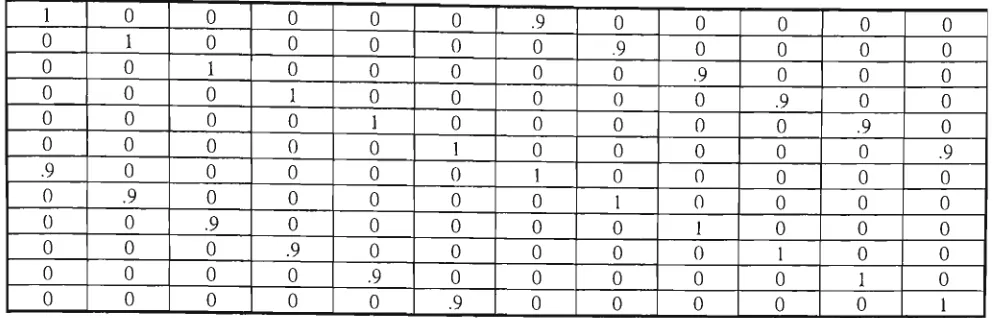
[ Z ( Q ) ] D = [ Z ( Q ) ] U D ® [ Q Z ] (2.2.5)

where the operator ® defines the element operation Z ( Q ) D y = Z(Q)UD y Qz y ;

Here the matrix [Q^] is denoted as damage quantification coefficient matrix due

to changes in both mass and stiffness. The use of the operator ® in equation

(2.2.5) ensures that all elements of dynamic stiffness matrix with values of zero

(48)

Z(Q)uD,ij has a value of zero, Z(Q)D y will also have a value of zero. As a result,

the connectivity of the undamaged and damaged structure remains the same.

If the difference in dynamic stiffness of the structure at a frequency Q due to

damage is denoted by [AZ(Q)], then

[ A Z ( Q ) ] = [Z(Q)]uD - [Z(a)]D (2.2.6)

Combining equations (2.2.5) and (2.2.6) together yields

[AZ(Q)] = [Z(Q)]UD - [Z(n)]uD ®[Qz] (2.2.7)

or [ A Z ( Q ) ] = [Z(Q)]uD ® ([U] - [U] ® [QJ) (2.2.8)

Following the method suggested by Kabe [8], any unrealistic changes in

dynamic stiffiiess elements can be minimized by defining an error function such

that it is independent of the magnitude of dynamic stiffness elements. This is

done by defining the error frmction as the norm of matrix ([U]- [U]®[Qz])

which can be denoted as:

e = ||[U]-[U](8)[Qj| (2.2.9)

e = S Z ( ^ - U , Q . , ) ^ (2.2.10)

where Uy = 1 if Z^D,]] ^ 0 and Uy = 0 if ZuD,ij = 0

From a mathematical viewpoint, the objective is to determine a matrix [Qz]

which will result in minimum deviation between the dynamic stiffiiess matrix

(49)

from equation (2.2.5), a known [Q^] will lead to the dynamic stiffiiess matrix

[Z(Q)]D. This mathematical operation needs to be performed under certain

physical constraints. These constraints ensure that the resultant dynamic

stiffness matrix (dynamic stiffness matrix corresponding to damaged structure)

satisfies the physical reality of the structure. If an adequate number of such

constraints can be imposed when determining [Qz], it is both mathematically

and physically feasible to expect that the dynamic stiffness matrix obtained will

represent the damaged structure. The mathematical formulation of the problem

is as follows:

Given a vector {ao(Q)}k which is the measured k column of receptance

matrix of the damaged structure, find a matrix [Qz] which minimizes the

norm given by equation (2.2.9) and also satisfies the constraints given by

equations (2.2.11) and (2.2.12) below:

([Z(Q)]uD® [Qz]){aD(^)}k- {S}k= {0} (2.2.11)

tVi

where {5}^ is a vector whose elements are zero except that the k element is

unity and

[Qz]-[Qzf=[0] (2.2.12)

From a physical viewpoint, the first constraint ensures that the calculated [Qz]

should be such that the dynamic stiffness derived is orthogonal to any column

of the receptance matrix of the damaged structure. The second constraint is

(50)

Structure is symmetric. Using the method of Lagrange Multipliers, as discussed

in appendix C, to incorporate these constraints, a Lagrange function can be

defined as:

L = e + :^gi + ^g2 (2.2.13)

where X and |LI are the Lagrange multipliers, gi and g2 are the given constraints

and L is the Lagrange function. It can be written as

n n

L = e + X ^ , ( Z Z ( Q ) ^ , Q , . , a , ^ , ) - Y + X Z ^ i , ( Q z , - Q z , , ) (2-2.14)

i=l 1=1 i=l j=l

where Y represents the second term on left hand side of equation (2.2.11).

Taking the partial derivative of L with respect to Qz^y and setting them equal to

zero yields an equation that Qz,y has to satisfy for L to be minimal:

Sy = - 2 ( U , , - Q , , , ) + X , Z ( n ) ™ , a „ j + H „ - H j , = 0 (2.2.15)

<5Qz,,

Equation (2.2.15) can be written in a matrix form yielding:

-2([U] - [Qz]) + [Z(Q)]uD® ({^}{ocD(^)}k^) + [l^] - il^f = [0] (2.2.16)

Since the physical constraints are applied at a single frequency Q, the Lagrange

multiplier has a single column corresponding to the frequency point used.

Taking the transpose of equation (2.2.16) and adding it to equation (2.2.16)

(51)

4([U] - [Qz]) + [Z(Q)]uD® ({^}{aD(Q)}/+ {a:,(Q)h{Xf) = [0] (2.2.17)

Multiplying equation (2.2.17) by 0 . 2 5 [ Z ( Q ) ] U D and rearranging terms it yields.

[Z(a)]uD® [Qz] = [ Z ( Q ) ] U D - [ZSQ] ® {{X}{a:,iQ)]J+ {ao(Q)k {X}^)}(2.2.18)

where [ZSQ] = 0 . 2 5 [ Z ( Q ) ] U D ® [Z(Q)]UD

Replacing equations (2.2.18) into (2.2.11), the following equation is derived:

[Z(Q)]uD{aD(n)}k- [ZSQ] (8) ({;V}{aD(a)}k^+ {aD(Q)}k{^}^){aD(Q)}k

= {6}k (2.2.19)

(2.2.20)

where {X} = ([Z(Q)]uD{aD(Q)}k - (Slk)

[ZSQ] 0 ({^}{aD(Q)}'^k+ {aD(^)}k {^}^){aD(Q)}k= {X}

Now the left hand side of equation (2.2.20) can be written as:

ZzSQ,a?,,„

i=l

0

SzSQ^.af,,,

i=l

hi

> +

ZSQ,,a],jo •• ZSQj„a„^Dan^p

Z S Q n i O t n k . D ^ l k . D ZSQ„nOCnk,D X,

x^

Hence equation (2.2.20) can be written as:

([a] + [b]){^} = {X}

-1

or, {;i}==([a]+[b])-'{X} (2.2.21)

Once {X} is derived, it can be put back into equation (2.2.18) to derive the

(52)

The dynamic stiffness matrix [Z(Q)] is a function of frequency. Therefore, at a

different frequency the matrix [Qz] will also be different, resulting in a different

error function defined in equation (2.2.9). The constraint equations will also be

frequency dependant.

However, if it is assumed that due to structural damage, only stiffiiess

characteristics have been affected, while variations in mass are small enough to

be neglected, then the error function may be simplified. In such case, it can be

written as

[AK] = [ K ] U D - [ K ] D (2.2.22)

or, [AK] = [K]UD([U] - [U] ® [QK]) (2.2.23)

where matrix [QK] is denoted as the damage quantification matrix due to change

in stiffhess only. Since the stiffhess matrix does not vary with frequency, the

constraint equations may be used repeatedly for multiple frequency points.

Therefore the constraint equation becomes :

( [ K ] u D ® [ Q K ] ) [ { a D ( ^ l ) } k v . . { a D ( n n ) } k ] " [ M ] u D [ { a D ( Q l ) } k v . . , { a D ( Q n ) } k ] [ ^ n ' ]

-[{5}k...{5}k] = [0] (2-2.24)

or, ( [ K ] U D ® [QK])[AD] - [M]uD[AD][^n'] - [{§}k, ,{S}k] - [0] (2.2.25)

where [ Q / ] is a diagonal matrix. Qj (i = 1, 2, ...., n) is the frequency at which

RFRF data have been measured, and

(53)

The second physical constraint is again the symmetry of matrix [Q^],

[QK] - [QK]'' - [0] (2.2.26)

The Lagrange function in equation (2.2.14) can then be defined as:

n s n

L = e + E S : ^ , ( Z K ^ , Q K , A O , )

-

Y + E Z ^ O ( Q K , ,

-

QK,,)

(2-2.27)

i=l j=l 1=1 i=l j=l

Here 's' represents the number of frequency points used. The term Y represents

the second and third terms of the left hand side of equation (2.2.25) which are

not a function of Q^ y and need not be defined. They do not contribute to the

derivative of L with respect to QK,ij.

Taking the partial derivative of L with respect to QK,y and setting them equal to

zero yields equations that Q^^ have to satisfy for L to be minimal. Repeating

the same procedure for the case of the dynamic stiffness matrix gives:

-2([U] - [QK]) + [K]uD® rniA^f) + M - [lif = [0] (2.2.28)

In contrast to equation (2.2.16), the constraint has been applied here at multiple

frequency points and hence the Lagrange multiplier is given by a matrix [k]

where each column corresponds to a particular frequency point. Adding the

transpose of equation (2.2.28) to itself yields :

(54)

Multiplying equation (2.2.29) by 0.25[K]UD and rearranging terms yields,

[K]uD® [QK] = [K]uD - 0.25 [KSQ] ® ( [ X ] [ A D ] ^ + [AD][^]^) (2.2.30)

where [KSQ] = [Kj^o ® [K]UD

Substituting equation (2.2.30) into equation (2.2.25) leads to :

[D] + {[KSQ] ® ([?.][AO]'')}[AD] + {[KSQ] (x) ([AD][;1]'")}[AD] = [0] (2.2.31)

where [D] = 4.0i[KU[Ah- [MU[AU Q„'] - [{5}k...{5}k])

Equation (2.2.31) can be used to establish [X] which when put back into

equation (2.2.30), will yield [K]^. From equation (2.2.31) the following

relationship can be derived

D} = ([T] + [S]){^} (2.2.32)

where the column vector {D} is formed by putting columns of [D] into a single

column consecutively. The same happens to column vector {X}. Matrix [T] can

be represented by the following matrix

[G']

.. 0