Non-perturbative determination of improvement b-coefficients in Nf = 3

Non-perturbative determination of improvement

b

-coefficients

in

N

=

3

Giulia Mariade Divitiis1,2,_{, Maurizio Firrotta}1,2_{, JochenHeitger}3_{, Carl ChristianKöster}3_{, and} AnastassiosVladikas2

1_{Dipartimento di Fisica, Università di Roma Tor Vergata, Via della Ricerca Scientifica 1, 00133 Rome, Italy} 2_{INFN, Sezione di Tor Vergata, c/o Dipartimento di Fisica, Università di Roma Tor Vergata, Via della Ricerca} Scientifica 1, 00133 Rome, Italy

3_{Institut für Theoretische Physik, Universität Münster, Wilhelm-Klemm-Str. 9, 48149 Münster, Germany}

Abstract. We present our preliminary results of the non-perturbative determination of the valence mass dependent coefficientsbA−bPand bm as well as the ratioZPZm/ZA

entering the flavour non-singlet PCAC relation in lattice QCD withNf =3 dynamical

flavours. We apply the method proposed in the past for quenched approximation and

Nf =2 cases, employing a set of finite-volume ALPHA configurations with Schrödinger

functional boundary conditions, generated withO(a) improved Wilson fermions and the

tree-level Symanzik-improved gauge action for a range of couplings relevant for simula-tions at lattice spacings of about 0.09 fm and below.

1 Introduction

Discretisation effects of lattice quantities computed with Wilson fermions are linear in the lattice

spac-inga, and may be a source of significant systematic errors, resulting in poor control of the continuum

extrapolations of physical observables. In the Symanzik improvement programme theseO(a) effects

can be removed by adding irrelevant operators both to the lattice action and to the local operators

in-serted in bare correlation functions. These so-called Symanzik counterterms have coefficients which

must be tuned non-perturbatively, in order to remove allO(a) contributions from physical quantities.

The improvement coefficients which multiply mass dependent Symanzik counterterms are referred in

the literature asb-coefficients. We will present preliminary results for theb-coefficients related to the

renormalised quark masses in QCD with three dynamical sea quarks. For analogous results on the

renormalisation and improvement of the vector current see Ref. [1].

2 Improvement condition

The improvement coefficients are short distance quantities. They can be determined by imposing

suitable conditions in small physical volumes. We adopt the Schrödinger functional setup, withL3_×T

lattices having periodic (Dirichlet) boundary conditions in space (time). The renormalisation scale is _{Talk given at the 35th International Symposium on Lattice Field Theory, 18-24 June 2017, Granada, Spain.}

µ=1/L. As we will exploit the freedom to keep sea- and valence-quark masses distinct, our setup

is non-unitary. Sea quark masses are tuned to the chiral limit, in line with the usual ALPHA choice

of a mass-independent renormalisation scheme. As the bare coupling g0 is varied, all other bare

parameters (such as the valence quark masses) are tuned so as to stay on a line of constant physics. This ensures that theb-coefficients are smooth functions ofg0.

The non-pertubative definition of theb-coefficients is not unique and depends upon the chosen

im-provement condition. The one we use is the standard non-singlet PCAC relation among renormalised quantities [2]:

˜

∂µ

ARi jµ(x)Oji

=(mR,i+mR,j)

PRi j(x)Oji

+O(a2), (1)

whereARi jµ, PRµi j,mR,i,mR,jdenote the renormalised axial current, pseudoscalar density and masses

with flavour indicesi, j. In the following, quantities with the same flavour index, such as A11

µ,m22 etc., are intended as defined for two distinct but degenerate valence flavours, so as to avoid Wick contractions that give rise to diagrams with disconnected quark lines. Improvement enforces this Ward identity, which holds in the continuum, to have no corrections linear in the lattice spacing, extending its validity up toO(a2_{) violations. Starting from the bare quantities}

Ai jµ ≡ψ¯iγµγ5ψj, Pi j≡ψ¯iγ5ψj,

mq,i j≡1₂(mq,i+mq,j), mq,i≡m0,i−mcrit= ₂1_a(_κ1_i −_κcrit1 ), (2)

we can write the renormalised masses and operators, in standard notation, as [3]:

ARi jµ =ZA(1+bAamq,i j+bA¯ atr ˆm(sea)_){Ai j

µ+cAa∂˜µPi j},

PRi jµ =ZP(1+bPamq,i j+bP¯ atr ˆm(sea)_)Pi j_{, (3)} mR,i=Zm

mq,i(1+bmamq,i+

¯

bmatr ˆm(sea))+xtr ˆm(sea)+yatr ˆm2(sea)+z a(tr ˆm(sea))2.

x≡(1−rm)/Nf y≡(rmdm−bm)/Nf z≡(rmd¯m−b¯m)/Nf

In small print we give the expressions forx, y andzin terms of the parameters rm,bm,bm¯ ,dm,dm¯

defined in Ref. [3]. It is important to keep in mind that the coefficientsbA,bP andbm, multiplying valence quark masses, arise from the mass dependence of the valence quark propagators and contain

also mass-independent contributions from the fermion loops. On the other hand ¯bA,bP¯ ,x, y,zarise

from the mass dependence of quark fermion loops. By keeping valence and sea quark masses distinct and tuning the bare (subtracted) sea-quark mass-matrix ˆm(sea)_{to the chiral limit, the above expressions}

simplify as indicated.

3 Non-perturbative definitions of

b

−

b

,

b

, and

Z

We compute Schrödinger functional correlation functions

f_Ai j(x0)≡ −a3

x

_Ai j

0(x)Oji,

f_Pi j(x0)≡ −a3

x

_Pi j_(x)Oji_{, O}ji_≡a6

u,v ¯

ζj(u)γ5ζi(v), (4)

with the operatorsA,Plocated in the bulk (0 < x0 <T) and the source operatorOji_{located on the}

µ=1/L. As we will exploit the freedom to keep sea- and valence-quark masses distinct, our setup

is non-unitary. Sea quark masses are tuned to the chiral limit, in line with the usual ALPHA choice

of a mass-independent renormalisation scheme. As the bare coupling g0 is varied, all other bare

parameters (such as the valence quark masses) are tuned so as to stay on a line of constant physics. This ensures that theb-coefficients are smooth functions ofg0.

The non-pertubative definition of theb-coefficients is not unique and depends upon the chosen

im-provement condition. The one we use is the standard non-singlet PCAC relation among renormalised quantities [2]:

˜

∂µ

ARi jµ(x)Oji

=(mR,i+mR,j)

PRi j(x)Oji

+O(a2), (1)

whereARi jµ,PRµi j,mR,i,mR,j denote the renormalised axial current, pseudoscalar density and masses

with flavour indicesi, j. In the following, quantities with the same flavour index, such as A11

µ,m22 etc., are intended as defined for two distinct but degenerate valence flavours, so as to avoid Wick contractions that give rise to diagrams with disconnected quark lines. Improvement enforces this Ward identity, which holds in the continuum, to have no corrections linear in the lattice spacing, extending its validity up toO(a2_{) violations. Starting from the bare quantities}

Ai jµ ≡ψ¯iγµγ5ψj, Pi j≡ψ¯iγ5ψj,

mq,i j≡1₂(mq,i+mq,j), mq,i≡m0,i−mcrit=₂1_a(_κ1_i −_κ1_crit), (2)

we can write the renormalised masses and operators, in standard notation, as [3]:

ARi jµ =ZA(1+bAamq,i j+bA¯ atr ˆm(sea)_){Ai j

µ+cAa∂˜µPi j},

PRi jµ =ZP(1+bPamq,i j+bP¯ atr ˆm(sea)_)Pi j_{, (3)} mR,i=Zm

mq,i(1+bmamq,i+

¯

bmatr ˆm(sea))+xtr ˆm(sea)+yatr ˆm2(sea)+z a(tr ˆm(sea))2.

x≡(1−rm)/Nf y≡(rmdm−bm)/Nf z≡(rmd¯m−b¯m)/Nf

In small print we give the expressions for x, y andz in terms of the parametersrm,bm,bm¯ ,dm,dm¯

defined in Ref. [3]. It is important to keep in mind that the coefficientsbA,bPandbm, multiplying valence quark masses, arise from the mass dependence of the valence quark propagators and contain

also mass-independent contributions from the fermion loops. On the other hand ¯bA,bP¯ ,x, y,zarise

from the mass dependence of quark fermion loops. By keeping valence and sea quark masses distinct and tuning the bare (subtracted) sea-quark mass-matrix ˆm(sea)_{to the chiral limit, the above expressions}

simplify as indicated.

3 Non-perturbative definitions of

b

−

b

,

b

, and

Z

We compute Schrödinger functional correlation functions

f_Ai j(x0)≡ −a3

x

_Ai j

0(x)Oji,

f_Pi j(x0)≡ −a3

x

_Pi j_(x)Oji_{, O}ji_≡a6

u,v ¯

ζj(u)γ5ζi(v), (4)

with the operatorsA,Plocated in the bulk (0< x0 <T) and the source operatorOji_{located on the}

boundary (x0 =0). We also compute the correlation functionsgi j_A,P(T −x0) with the same operator

insertions in the bulk and sourcesOji_{at (x}

0 =T). Due to the symmetric boundary conditions on the

gauge fields, we can symmetrisef_Ai j_,Pandgi j_A,P, thus reducing statistical fluctuations. The

renormalisa-tion pattern and improvement constraint imply that the current (PCAC) massmi j, defined by

mi j(x0)≡

˜

∂0f_Ai j(x0)+acA∂∗₀∂0f_Pi j(x0)

2 f_Pi j(x0) , (5)

can be parametrised as

mi j(x0)=Z

xtr ˆm(sea)₊

[z+x(b¯_A−b¯_P)]a(tr ˆm(sea))2+yatr ˆm2(sea) ₍₆₎

+mq,i j(1+[x

(bA−bP)+b¯m−(b¯A−b¯P)]atr ˆm(sea))+am2_{q,i j}(bP−bA)+1₂a(m2_q,i+m2_q,j)bm,

where the slashed terms nearly vanish at ˆm(sea)_{≈0 andZ indicates the ratio of renormalisation}

con-stantsZ(g2₀) ≡ Zm(g2₀,a/L)ZP(g2₀,a/L)/ZA(g2₀). For the various lattice derivatives standard notation

is used: symmetric ˜∂, forward ∂, backward ∂∗. Nearest-neighbour derivatives ˜∂ and ∂∗∂ suffer

fromO(a2_{) discretisation errors; we label results produced with them with “standard derivative”.}

In Refs. [4,5], next-to-nearest-neighbour definitions have been proposed, withO(a4_{) errors. Results}

obtained with these definitions are labelled with “improved derivative”.

We determine the improvement coefficients adopting the same strategy introduced for quenched

QCD in [4–7] and applied later for the two flavour case [8]. We consider three different valence

flavoursi,j =1,2,3 and compute the four different PCAC massesm11,m22,m33,m12. Up to

renor-malisation, these are physical quantities. We keepm11andm22fixed along our line of constant physics.

The hopping parameterκ1of the first valence flavour is set equal to the value of the dynamical quarks,

in order to have nearly vanishigm11. For the second valence flavour, κ2 is chosen so that m22 is

approximately equal to four arbitrary reference values:

Lm11≈0.0,

Lm22≈0.25,0.5,0.75,1.0. (7)

The third flavour is such that the corresponding bare mass is halfway the two others:

m0,3=1₂(m0,1+m0,2), equivalently mq,3=1₂(mq,1+mq,2). (8)

The renormalisation and improvement structure of PCAC mass differences is as follows:

      

∆₂₂,11 ≡1₂(m22−m11) =Zδ

1+aA(sea)+2am¯b_mAP+. . . ∆₂₂,33 ≡(m22−m33) =Zδ

1+aA(sea)+(2am¯ +aδ)bmAP+. . . ∆₃₃,11 ≡(m33−m11) =Zδ

1+aA(sea)+(2am¯ −aδ)bmAP+. . . ∆₂₂,12 ≡(m22−m12) =Zδ

1+aA(sea)+2am¯bmAP₋aδbAP+. . . ∆₁₂,11 ≡(m12−m11) =Zδ

1+aA(sea)+2am¯bmAP+aδbAP+. . . ,

(9)

am¯ ≡amq,2+amq,1

/2, aδ≡amq,2−amq,1

/2,

BothaA(sea)_{andZcancel in the ratio of mass differences, enabling us to single outb}

A−bP,bm, as well

asZ:

RAP ≡(2m12−m11−m22) ∆amq,2−amq,1

=b_A−b_P+O(amq,1+amq,2),

Rm≡ 2 (m12−m33) ∆amq,2−amq,1

= b_m+O(amq,1+amq,2), (10)

RZ ≡_mm11−m22

q,1−mq,2 +(RAP−Rm) (am11+am22)=Z+O(atr ˆm (sea)_).

In the above expressions,∆without subscripts indicates any of the five ∆’s in Eqs. (9), leading to

five possible determinations of theb’s, which differ byO(a) terms. This ambiguity becomesO(a2)

when theb’s are inserted in the definition of renormalised, improved quark-masses. With exactly

massless sea quarks the ambiguity inZ isO(a2_{). These formulae generalise the ones in previous}

works [4,5,7,8].

4 Simulation details

As already mentioned, our simulations are performed on a constant-physics trajectory in the space

of bare parameters, with all physical scales held fixed, as illustrated in Fig.1. We use the gauge

configurations generated by the ALPHA collaboration, with the coupling constantβ=6/g2₀tuned so

that the physical lattice extent is fixed toL ≈1.2 fm. The tuning is based on the 2-loop perturbative

expression for the lattice spacing. Subsequently, the value ofκ (corresponding to the mass of the

degenerate sea quarks) is fixed for each lattice, so as to obtain a vanishing PCAC mass. The parameters

of the available configurations are shown in Tab. 1. The values ofβspan a range which is suitable

for large-volume simulations. They correspond to the interval of lattice spacings 0.045 fm a

0.090 fm. All lattices (except E1k1 and E1k2 whereT =3L/2) have temporal sizeT =3L/2₋a. For

details, see Ref. [9,10].

L

T=3L/2−a

A1k1, A1k2 B1k1, B1k2, B1k3, B2k1 C1k2, C1k3 D1k1

Figure 1.Lattices with varying lattice spacing but identical physical sizeL≈1.2 fm.

The SF simulations have been performed using theopenQCDcode [11], with improved Lüscher–

Weisz gauge action [12],Nf =3 massless Wilson-clover fermions, vanishing boundary gauge fields

C=C=0 and boundary fermion parameterθ=0. The value of the improvement coefficientcSWis

taken from Ref. [13]. The RHMC algorithm [14–16] is used for the third dynamical quark.

5 Results

BothaA(sea)_{andZcancel in the ratio of mass differences, enabling us to single outb}

A−bP,bm, as well

asZ:

RAP ≡(2m12−m11−m22) ∆amq,2−amq,1

=b_A−b_P+O(amq,1+amq,2),

Rm≡ 2 (m12−m33) ∆amq,2−amq,1

= b_m+O(amq,1+amq,2), (10)

RZ ≡_mm11−m22

q,1−mq,2 +(RAP−Rm) (am11+am22)=Z+O(atr ˆm (sea)_).

In the above expressions,∆without subscripts indicates any of the five∆’s in Eqs. (9), leading to

five possible determinations of theb’s, which differ byO(a) terms. This ambiguity becomesO(a2)

when theb’s are inserted in the definition of renormalised, improved quark-masses. With exactly

massless sea quarks the ambiguity inZ isO(a2_{). These formulae generalise the ones in previous}

works [4,5,7,8].

4 Simulation details

As already mentioned, our simulations are performed on a constant-physics trajectory in the space

of bare parameters, with all physical scales held fixed, as illustrated in Fig.1. We use the gauge

configurations generated by the ALPHA collaboration, with the coupling constantβ=6/g2₀tuned so

that the physical lattice extent is fixed toL≈1.2 fm. The tuning is based on the 2-loop perturbative

expression for the lattice spacing. Subsequently, the value ofκ (corresponding to the mass of the

degenerate sea quarks) is fixed for each lattice, so as to obtain a vanishing PCAC mass. The parameters

of the available configurations are shown in Tab.1. The values ofβspan a range which is suitable

for large-volume simulations. They correspond to the interval of lattice spacings 0.045 fm a

0.090 fm. All lattices (except E1k1 and E1k2 whereT =3L/2) have temporal sizeT =3L/2₋a. For

details, see Ref. [9,10].

L

T=3L/2−a

A1k1, A1k2 B1k1, B1k2, B1k3, B2k1 C1k2, C1k3 D1k1

Figure 1.Lattices with varying lattice spacing but identical physical sizeL≈1.2 fm.

The SF simulations have been performed using theopenQCDcode [11], with improved Lüscher–

Weisz gauge action [12],Nf =3 massless Wilson-clover fermions, vanishing boundary gauge fields

C =C=0 and boundary fermion parameterθ=0. The value of the improvement coefficientcSWis

taken from Ref. [13]. The RHMC algorithm [14–16] is used for the third dynamical quark.

5 Results

The preliminary results presented in the this work are obtained from the analysis of the B1k3 ensem-ble, marked in red in Tab.1.

Table 1. Simulation parametersL,T, β, κ, number of replicas # REP (i.e. number of statistically independent sets of configurations from Monte Carlo runs at identical parameters) and number of molecular dynamics units

# MDU for each ensemble ID.

L3_×T/a4 _{β κ # REP # MDU ID}

123_{×17 3.3 0.13652 10 10240 A1k1}

0.13660 10 12620 A1k2 143_{×21 3.414 0.13690 32 10360 E1k1}

0.13695 48 13984 E1k2

163_{×23 3.512 0.13700 2 20480 B1k1}

0.13703 1 8192 B1k2

0.13710 3 24560 B1k3

163_{×23 3.47 0.13700 3 29584 B2k1}

203_{×29 3.676 0.13700 4 15232 C1k2}

0.13719 4 15472 C1k3 243_{×35 3.810 0.13712 5 10240 D1k1}

The time dependence of the PCAC massesm11,m22,m33,m12is shown in Fig.2. These results are

obtained with improved derivatives; those obtained with standard derivatives do not show appreciable

differences. All masses show wide plateaux, and the statistical errors are smaller than the symbols.

The red points correspond to the chiral flavourm11 ≈0, while the blue data representm22. As can

be seen on the right vertical axis, m22 is tuned with good precision to the chosen reference values

Lm22≈0.25,0.5,0.75,1.0 of Eq. (7).

-0.02 0 0.02 0.04 0.06 0.08 0.1

0 5 10 15 20

-0.25 0 0.25 0.5 0.75 1 1.25

am Lm

x₀/a

impr deriv

m11

m12

m33

m22

Figure 2.Time dependence of PCAC masses for the ensemble B1k3.

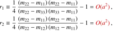
To check the consistency of our data with the parametrisation of the cutoffeffects given in Eqs. (9),

we verify that the quantities

r1≡1₄ (_(m22m22−m11) (m22−m11)

−m33) (m33−m11) −1=O(a2),

r2≡1₄ (_(m22m22−m11) (m22−m11)

−m12) (m12−m11) −1=O(a2), (11)

are close to zero. As can be seen in Fig. 3, these ratios are of order 10−4 _{and less, significantly}

smaller than the valuesamq,2≈0.015,0.06, with improved-derivative data having the smaller values.

r2demonstrates that results for theb’s are insensitive to the choice of∆in the denominator. In what

follows we set∆ = ∆₂₂,11, which is the one kept fixed on the line of constant physics.

0 4 8 12 16 20 x0/a

L m22=0.75

0 4 8 12 16 20 -0.0002 0 0.0002 0.0004 0.0006 0.0008

x0/a L m22=1.0

-0.0002 0 0.0002 0.0004 0.0006 0.0008

0 4 8 12 16 20

r1

x0/a

L m22=0.25

0 4 8 12 16 20 x0/a

L m22=0.5

(a)r1.

0 4 8 12 16 20 x0/a

L m22=0.75

0 4 8 12 16 20 -0.0002 0 0.0002 0.0004 0.0006 0.0008

x0/a L m22=1.0

-0.0002 0 0.0002 0.0004 0.0006 0.0008

0 4 8 12 16 20

r2

x0/a

L m22=0.25

0 4 8 12 16 20 x0/a

L m22=0.5

(b)r2.

Figure 3. Time dependence of the ratiosr1 andr2for the ensemble B1k3. Blue points refer to PCAC masses

computed with standard derivatives, red points to those computed with improved ones. The four plots correspond to the four reference valuesLm22=0.25,0.5,0.75,1.0.

The main results of our preliminary analysis are presented in Fig.4. The plots (a),(b) and (c) show

the time dependence of estimators forbAP,bmandZ, respectively, with blue points corresponding to

the standard derivative and red points to the improved one. The horizontal lines in the plots indicate

the averages over the time windowx0/a=[8; 15], corresponding to the middle third of the time extent

T. Averaging over time slices is part of our operative definition of the parametersbAP,bm,Z. Note that

RAPdata show a significant ambiguity with respect to the choice of the lattice derivative, as previously

observed in the quenched andNf =2 studies [4,5,8].

In general all signals show better plateaux and smaller statistical errors at larger values ofm22,

where however discretisation effects are expected to be larger.

5.1 Topological sectors

Since Ward identities hold in any topological sector and the improvement coefficients are short

dis-tance quantities, our results should be insensitive to the topological chargeQ. Following Ref. [9],

we repeated our data analysis only considering configurations belonging to the trivial (i.e. Q = 0)

topological sector, using a topological charge defined through gradient-flow fields [17,18]

Q(t)≡ −₃₂a4_π2 x

µναβtr{Gµν(x,t)Gαβ(x,t)}, Gµν ≡∂µBν−∂νBµ+[Bµ,Bν], (12)

wheretis the flow time, kept fixed in units of physical volume, andBµis the gluon field. The results

r2demonstrates that results for theb’s are insensitive to the choice of∆in the denominator. In what

follows we set∆ = ∆₂₂,11, which is the one kept fixed on the line of constant physics.

0 4 8 12 16 20 x0/a

L m22=0.75

0 4 8 12 16 20 -0.0002 0 0.0002 0.0004 0.0006 0.0008

x0/a L m22=1.0

-0.0002 0 0.0002 0.0004 0.0006 0.0008

0 4 8 12 16 20

r1

x0/a

L m22=0.25

0 4 8 12 16 20 x0/a

L m22=0.5

(a)r1.

0 4 8 12 16 20 x0/a

L m22=0.75

0 4 8 12 16 20 -0.0002 0 0.0002 0.0004 0.0006 0.0008

x0/a L m22=1.0

-0.0002 0 0.0002 0.0004 0.0006 0.0008

0 4 8 12 16 20

r2

x0/a

L m22=0.25

0 4 8 12 16 20 x0/a

L m22=0.5

(b)r2.

Figure 3. Time dependence of the ratiosr1andr2for the ensemble B1k3. Blue points refer to PCAC masses

computed with standard derivatives, red points to those computed with improved ones. The four plots correspond to the four reference valuesLm22=0.25,0.5,0.75,1.0.

The main results of our preliminary analysis are presented in Fig.4. The plots (a),(b) and (c) show

the time dependence of estimators forbAP,bmandZ, respectively, with blue points corresponding to

the standard derivative and red points to the improved one. The horizontal lines in the plots indicate

the averages over the time windowx0/a=[8; 15], corresponding to the middle third of the time extent

T. Averaging over time slices is part of our operative definition of the parametersbAP,bm,Z. Note that

RAPdata show a significant ambiguity with respect to the choice of the lattice derivative, as previously

observed in the quenched andNf =2 studies [4,5,8].

In general all signals show better plateaux and smaller statistical errors at larger values ofm22,

where however discretisation effects are expected to be larger.

5.1 Topological sectors

Since Ward identities hold in any topological sector and the improvement coefficients are short

dis-tance quantities, our results should be insensitive to the topological chargeQ. Following Ref. [9],

we repeated our data analysis only considering configurations belonging to the trivial (i.e. Q = 0)

topological sector, using a topological charge defined through gradient-flow fields [17,18]

Q(t)≡ −₃₂a4_π2 x

µναβtr{Gµν(x,t)Gαβ(x,t)}, Gµν ≡∂µBν−∂νBµ+[Bµ,Bν], (12)

wheretis the flow time, kept fixed in units of physical volume, andBµis the gluon field. The results

were in agreement with the full statistics (i.e. including all topological charges), while only reflecting fluctuations consistent with the reduction of statistics. This confirms the aforementioned expectation of the results’ insensitivity to topology.

0 4 8 12 16 20 x0/a

L m22=0.75

0 4 8 12 16 20 -1.5 -1 -0.5 0 0.5 1

x0/a L m22=1.0

-1.5 -1 -0.5 0 0.5 1

0 4 8 12 16 20

RAP

x0/a

L m22=0.25

0 4 8 12 16 20 x0/a

L m22=0.5

(a)RAP.

0 4 8 12 16 20 x0/a

L m22=0.75

0 4 8 12 16 20 -1 -0.8 -0.6 -0.4 -0.2 0 0.2 0.4

x0/a L m22=1.0

-1 -0.8 -0.6 -0.4 -0.2 0 0.2 0.4

0 4 8 12 16 20

Rm

x0/a

L m22=0.25

0 4 8 12 16 20 x0/a

L m22=0.5

(b)Rm.

0 4 8 12 16 20 x0/a

L m22=0.75

0 4 8 12 16 20 0.9 0.95 1 1.05 1.1

x0/a L m22=1.0

0.9 0.95 1 1.05 1.1

0 4 8 12 16 20

RZ

x0/a

L m22=0.25

0 4 8 12 16 20 x0/a

L m22=0.5

(c)RZ.

Figure 4. Time dependence ofRAP, Rm andRZ for the ensemble B1k3. Blue points refer to PCAC masses computed with standard derivatives, red points to those computed with improved ones. The four plots correspond to the four reference valuesLm22=0.25,0.5,0.75,1.0.

6 Conclusion

To complete our work we will compute the correlation functions for full statistics and on all

avail-able lattices at different lattice spacings (see Tab. 1). Combining the known analytic perturbative

expressions for these quantities, valid towards vanishingg2₀, with our data points, we aim at obtaining

suitable interpolation functions forbAP(g20),bm(g20), andZ(g20). These non-perturbative formulae are

needed for reachingO(a) improved results in simulations of lattice QCD withNf =3 Wilson quarks

in large volume. It will be interesting to compare our results to those recently obtained by Korcyl and Bali [19], using a different non-perturbative renormalisation method.

Acknowledgements

Computer resources were provided by the INFN (GALILEO cluster at CINECA) and the ZIV of the

University of Münster (PALMA HPC cluster). This work was supported by the grant HE 4517/3-1

(J. H.) of the Deutsche Forschungsgemeinschaft. C. C. K., scholar of the German Academic Scholar-ship Foundation (Studienstiftung des deutschen Volkes), gratefully acknowledges their financial and

academic support. The speaker wishes to thank Isabel Campos, Elvira Gámiz and all the organizers

References

[1] J. Heitger, F. Joswig, A. Vladikas, C. Wittemeier (ALPHA),Non-perturbative determination of

cV,ZV and ZS/ZP in Nf = 3 lattice QCD, inProceedings, 35th International Symposium on

Lattice Field Theory (Lattice2017): Granada, Spain, to appear in EPJ Web Conf.

[2] M. Lüscher, S. Sint, R. Sommer, P. Weisz, U. Wolff, Nucl. Phys. B491, 323 (1997),

hep-lat/9609035

[3] T. Bhattacharya, R. Gupta, W. Lee, S.R. Sharpe, J.M. Wu, Phys.Rev. D73, 034504 (2006),

hep-lat/0511014

[4] G.M. de Divitiis, R. Petronzio, Phys. Lett.B419, 311 (1998),hep-lat/9710071

[5] M. Guagnelli, R. Petronzio, J. Rolf, S. Sint, R. Sommer, U. Wolff(ALPHA), Nucl. Phys.B595,

44 (2001),hep-lat/0009021

[6] J. Heitger, J. Wennekers (ALPHA), JHEP02, 064 (2004),hep-lat/0312016

[7] T. Bhattacharya, R. Gupta, W.J. Lee, S.R. Sharpe, Phys. Rev. D63, 074505 (2001),

hep-lat/0009038

[8] P. Fritzsch, J. Heitger, N. Tantalo (ALPHA), JHEP08, 074 (2010),1004.3978

[9] J. Bulava, M. Della Morte, J. Heitger, C. Wittemeier (ALPHA), Nucl. Phys.B896, 555 (2015),

1502.04999

[10] J. Bulava, M. Della Morte, J. Heitger, C. Wittemeier (ALPHA), Phys. Rev.D93, 114513 (2016),

1604.05827

[11] openQCD, Simulation program for lattice QCD,http://luscher.web.cern.ch/luscher/openQCD/

[12] M. Lüscher, P. Weisz, Commun. Math. Phys. 97, 59 (1985), [Erratum: Commun. Math.

Phys.98,433 (1985)]

[13] J. Bulava, S. Schaefer, Nucl. Phys.B874, 188 (2013),1304.7093

[14] A.D. Kennedy, I. Horvath, S. Sint, Nucl. Phys. Proc. Suppl.73, 834 (1999),hep-lat/9809092

[15] M.A. Clark, A.D. Kennedy, Phys. Rev. Lett.98, 051601 (2007),hep-lat/0608015

[16] M. Lüscher, F. Palombi, PoSLATTICE2008, 049 (2008),0810.0946

[17] M. Lüscher, JHEP08, 071 (2010), [Erratum: JHEP03,092 (2014)],1006.4518

[18] M. Lüscher, P. Weisz, JHEP02, 051 (2011),1101.0963