Article
1
Deep Learning for Detecting Building Defects Using
2
Convolutional Neural Networks
3
Husein Perez *, Joseph H. M. Tah and Amir Mosavi
4
Oxford Institute for Sustainable Development, School of the Built Environment, Oxford Brookes
5
University, Oxford OX3 0BP, UK; [email protected] & [email protected]
6
* Correspondence: [email protected]
7
Abstract: Clients are increasingly looking for fast and effective means to quickly and frequently
8
survey and communicate the condition of their buildings so that essential repairs and maintenance
9
work can be done in a proactive and timely manner before it becomes too dangerous and expensive.
10
Traditional methods for this type of work commonly comprise of engaging building surveyors to
11
undertake a condition assessment which involves a lengthy site inspection to produce a systematic
12
recording of the physical condition of the building elements, including cost estimates of immediate
13
and projected long-term costs of renewal, repair and maintenance of the building. Current asset
14
condition assessment procedures are extensively time consuming, laborious, and expensive and
15
pose health and safety threats to surveyors, particularly at height and roof levels which are difficult
16
to access. This paper aims at evaluating the application of convolutional neural networks (CNN)
17
towards an automated detection and localisation of key building defects, e.g., mould, deterioration,
18
and stain, from images. The proposed model is based on pre-trained CNN classifier of VGG-16 (later
19
compaired with ResNet-50, and Inception models), with class activation mapping (CAM) for object
20
localisation. The challenges and limitations of the model in real-life applications have been
21
identified. The proposed model has proven to be robust and able to accurately detect and localise
22
building defects. The approach is being developed with the potential to scale-up and further
23
advance to support automated detection of defects and deterioration of buildings in real-time using
24
mobile devices and drones.
25
Keywords: deep learning; convolutional neural networks (CNN); transfer learning; class activation
26
mapping (CAM); building defects; structural-health monitoring
27
28
1. Introduction
29
Clients with multiple assets are increasingly requiring intimate knowledge of the condition of
30
each of their operational assets to enable them to effectively manage their portfolio and improve
31
business performance. This is being driven by the increasing adverse effects of climate change,
32
demanding legal and regulatory requirements for sustainability, safety and well-being, and
33
increasing competitiveness. Clients are looking for fast and effective means to quickly and frequently
34
survey and communicate the condition of their buildings so that essential maintenance and repairs
35
can be done in a proactive and timely manner before it becomes too dangerous and expensive [1-4].
36
Traditional methods for this type of work commonly comprise of engaging building surveyors to
37
undertake a condition assessment which involves a lengthy site inspection resulting in a systematic
38
recording of the physical conditions of the building elements with the use of photographs, note
39
taking, drawings and information provided by the client [5-7]. The data collected are then analysed
40
to produce a report that includes a summary of the condition of the building and its elements [8].
41
This is also used to produce estimates of immediate and projected long-term costs of renewal, repair
42
and maintenance of the building [9, 10]. This enables facility managers to address current operational
43
requirements, while also improving their real estate portfolio renewal forecasting and addressing
44
funding for capital projects [11]. Current asset condition assessment procedures are extensively time
45
consuming, laborious and expensive, and pose health and safety threats to surveyors, particularly at
46
height and roof levels which are difficult to access for inspection [12].
47
Image analysis techniques for detecting defects have been proposed as an alternative to the
48
manual on-site inspection methods. Whilst the latter is time-consuming and not suitable for
49
quantitative analysis, image analysis-based detection techniques, on the other hand, can be quite
50
challenging and fully dependent on the quality of images taken under different real-world situations
51
(e.g. light, shadow, noise, etc.). In recent years, researchers have experimented with the application
52
of a number of soft computing and machine learning-based detection techniques as an attempt to
53
increase the level of automation of asset condition inspection [14-20]. The notable efforts include;
54
structural health monitoring with Bayesian method [13], surface crack estimation using Gaussian
55
regression, support vector machines (SVM), and neural networks [14], SVM for wall defects
56
recognition [15], crack-detection on concrete surfaces using deep belief networks (DBN) [16], crack
57
detection in oak flooring using ensemble methods of random forests (RF) [17], deterioration
58
assessment using fuzzy logic [18], defect detection of ashlar masonry walls using logistic regression
59
[19-20]. The literature also includes a number of papers devoted to the detection of defects in
60
infrastructural assets such as cracks in road surfaces, bridges, dams, and sewerage pipelines [21–30].
61
The automated detection of defects in earthquake damaged structures has also received considerable
62
attention amongst researchers in recent years [31–33]. Considering these few studies, far too little
63
attention has been paid to the application of advanced machine learning methods and deep learning
64
methods in the advancements of smart sensors for the building defects detection. There is a general
65
lack of research in the automated condition assessment of buildings; despite they represent a
66
significant financial asset class.
67
The major objective of this research has therefore is set to investigate the novel application of
68
deep learning method of convolutional neural networks (CNN) in automating the condition
69
assessment of buildings. The focus is to automated detection and localisation of key defects arising
70
from dampness in buildings from images. However, as the first attempt to tackle the problem, this
71
paper applies a number of limitations. Firstly, multiple types of the defects are not considered at once.
72
This means that the images considered by the model belong to only one category. Secondly, only the
73
images with visible defects are considered. Thirdly, consideration of the extreme lighting and
74
orientation, e.g., low lighting, too bright images are not included in this study. In the future works,
75
however, these limitations will be considered to be able to get closer to the concept of a fully
76
automated detection.
77
The rest of this paper is organized as follows. A brief discussion of a selection of the most
78
common defects that arise from the presence of moisture and dampness in buildings is presented.
79
This is followed by a brief overview of CNN. These are a class of deep learning techniques primarily
80
used for solving fundamental problems in computer vision. This provides the theoretical basis of the
81
work undertaken. We propose a deep learning-based detection and localisation model using transfer
82
learning utilising the VGG-16 model [40] for feature extraction and classification. Next, we briefly
83
discuss the localisation problem and the class activation mapping (CAM) [41] technique which we
84
incorporated with our model for defect localisation. This is followed by a discussion of the dataset
85
used, the model developed, the results obtained, conclusions and future work.
86
87
2. Dampness in Buildings
88
Buildings are generally considered durable because of their ability to last hundreds of years.
89
However, those that survive long have been subject to care through continuous repair and
90
maintenance throughout their lives. All building components deteriorate at varying rates and
91
degrees depending on the design, materials and methods of construction, quality of workmanship,
92
environmental conditions and the uses of the building. Defects result from the progressive
93
deterioration of the various components that make up a building. Defects occur through the action
94
of one or a combination of external forces or agents. These have been classified in ISO 19208 [34] into
95
vibration and noises); electro-magnetic agents (e.g. solar radiation, radioactive radiation, lightening,
97
magnetic fields); thermal agents (e.g. heat, frost); chemical agents (water, solvents, oxidising agents,
98
sulphides, acids, salts); and biological agents (e.g. vegetable, microbial, animal). Carillion [35]
99
presents a brief description of the salient features of these five groups followed by a detailed
100
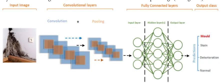
description of numerous defects in buildings including symptoms, investigations, diagnosis and
101
cure. Defects in buildings have been the subject of investigation over a number of decades and details
102
can be found in many standard texts [36–39].
103
Dampness is increasingly significant as the value of a building can be affected even where only
104
low levels of dampness are found. It is increasing seen as a health hazard in buildings. The fabric of
105
buildings under normal conditions contains a surprising amount of moisture which does not cause
106
any harm. The term dampness is commonly reserved for conditions under which moisture is present
107
in sufficient quantity to become either perceptive to sight or by touch, or to cause deterioration in the
108
decorations and eventually in the fabric of the building [42]. A building is considered to be damp
109
only if the moisture becomes visible through discoloration and staining of finishes, or causes mould
110
growth on surfaces, sulphate attack or frost damage, or even drips or puddles [42]. All of these signs
111
confirm that other damage may be occurring.
112
There are various forms of decay which commonly afflict the fabric of buildings which can be
113
attributed to the presence of excessive dampness. Dampness is thus, a catalyst for a whole variety of
114
building defects. Corrosion of metals, fungal attack of timber, efflorescence of brick and mortar,
115
sulphate attack of masonry materials, and carbonation of concrete are all triggered by moisture.
116
Moisture in buildings is a problem because it expands and contracts with temperature fluctuations,
117
causing degradation of materials over time. Moisture in buildings contains a variety of chemical
118
elements and compounds carried up from the soil or from the fabric itself which can attack building
119
materials physically or chemically. Damp conditions encourage the growth of wood rutting fungi,
120
the infestation of timber by wood boring insects and the corrosion of metals. It enables the house dust
121
mite population to multiply rapidly and moulds to grow, creating conditions which are
122
uncomfortable or detrimental to the health of occupants.
123
2.1 The Causes of Dampness
124
A high proportion of dampness problems are caused by condensation, rain penetration, and
125
rising damp [43]. Condensation occurs when warm air in the atmosphere reverts to water when it
126
comes into contact with cold surfaces that are below the dew-point temperature. It is most prevalent
127
in winter when activities such as cooking, showering and central heating release warm moisture into
128
the air inside the building. The condensate can be absorbed by porous surfaces or appear as tiny
129
droplets on hard shiny surfaces. Thus, condensation is dependent on the temperature of surfaces and
130
the humidity of the surrounding air. Condensation is the most common damp that can be found in
131
both commercial and residential property.
132
Rain penetration occurs mostly through roofs and walls exposed to the prevailing wind-driven
133
rainfall, with openings that permit its passage and forces to drive or draw it inwards. It can be caused
134
by the effects of incorrect design, bad workmanship, and structural movement, the wrong choice of
135
or decay of material, badly executed repairs or lack of regular maintenance [44]. The most exposed
136
parts of a building such as roofs, chimneys and parapets are the most susceptible to rain penetration.
137
Rising damp occurs through the absorption of water, by a physical process called capillary
138
action, at the lower sections of walls and ground supported structures that are in contact with damp
139
soil. The absorbed moisture rises to a height at which there is a balance between the rate of
140
evaporation and the rate at which it can be drawn up by capillary action [44]. Rising damp is
141
commonly found in older properties where the damp proof course is damaged or is absent. Other
142
causes of dampness include: construction moisture; pipe leakage; leakage at roof features and
143
abutments; spillage; ground and surface water; and contaminating salts in solution.
144
Moisture can damage the building structure, the finishing and furnishing materials and can
146
increase the heat transfer through the envelope and thus the overall building energy consumption
147
[25]. It may also cause a poor indoor air quality and respiratory illness in occupants [42]. In the main,
148
the types of deterioration driven by water in building materials include: moulds and fungal growth;
149
materials spalling; blistering; shrinkage; cracking and crazing; irreversible expansion; embrittlement;
150
strength loss; staining or discolouration; steel and iron rusting; and decay from micro-organisms. In
151
extreme cases, mortar or plaster may fall away from the affected wall. The focus of this paper is on
152
moulds, stains and paint deterioration which are the most common interrelated defects arising from
153
dampness.
154
Moulds and fungi occur on interior and exterior surfaces of buildings following persistent
155
condensation or other forms of frequent dampness. On internal surfaces, they are unsightly and can
156
cause a variety of adverse health effects including respiratory problems in susceptible individuals
157
[42]. Moulds on external surfaces are also unsightly and cause failure of paint films. Fungi growth
158
such as algae, lichens and mosses generally occur on external surfaces where high moisture levels
159
persist for long periods [45,46]. They are unsightly and can cause paint failure like moulds.
160
Paint deterioration typically occurs on building surfaces exposed to excessive moisture,
161
dampness and other factors due to anthropogenic activity. The daily and seasonal variations in
162
temperatures that oscillate between cold and warm, cause the moisture to expand and contract
163
continuously resulting in paint slowly separating from a building’s surface. The growth of mildew
164
and fungi in the presence of moisture and humid conditions will cause paint damage. The exposure
165
of exterior surfaces to sun and its ultra-violet radiation causes paint to fade and look dull. Exposure
166
to airborne salts and pollution will also cause paint deterioration. Paint deterioration is visible in the
167
form of peeling, blistering, flacking, blooming, chalking, and crazing.
168
3. Convolutional Neural Networks (ConvNet)
169
CNN, a class of deep learning techniques, are primarily used for solving fundamental problems
170
in computer vision such as image classification [47], object detection [23,48], localisation [25] and
171
segmentation [49]. Although early deep neural networks (DNN) go back to the 1980’s when
172
Fukushima [50] applied them for visual pattern recognition, they were not widely used, except in few
173
applications, mainly due to limitation in the computational power of the hardware which is needed
174
to train the network. It was in mid-2000s when the developments in computing power and the
175
emergence of large amounts of labelled datasets contributed to deep learning advancement and
176
brought CNN back to light [51].
177
3.1 CNN Architecture
178
The simplest form of a neural network is called perceptron. This is a single-layer neural network
179
with exactly one input layer and one output layer. Multiple perceptrons can be connected together
180
to form a multi-layer neural network with one input, one output and multiple inner layers, which
181
also known as hidden layers. The more hidden layers, the deeper is the neural network (hence the
182
name deep neural network) [52]. As a rule of thumb when designing a neural network, the number
183
of nodes in the input layer is equal to the number of features in the input data, e.g. since our inputs
184
are images with 3-channel (Red, Green, Blue) with 224x 224 pixels in each channel, therefore, the
185
number of nodes in our input layer is 3x224x224. The number of nodes in the output layer, on the
186
other hand, is determined by the configuration of the neural network. For example, if the neural
187
network is a classifier, then the output layer needs one node per class label, e.g. in our neural network,
188
we have four nodes corresponding to the four class labels: mould, stain, deterioration and normal.
189
When designing a neural network, there are no particular rules that govern the number of
190
hidden layers needed for a particular task. One consensus on this matter is how the performance
191
changes when adding additional hidden layers, i.e. the situations in which performance improves or
192
driven” rules of thumbs about the number of nodes (the size) in each hidden layer [54]. One common
194
way suggest that the optimal size of the hidden layer should be between the size of the input layer
195
and the size of the output layer [55].
196
3.1.1 CNN Layers
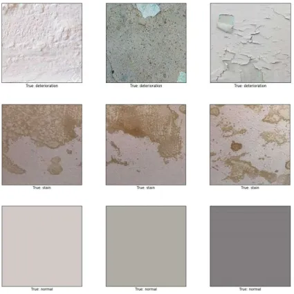
197
Although, CNN have different architectures, almost all follow the same general design
198
principles of successively applying convolutional layers and pooling layers to an input image. In such
199
arrangement, the ConvNet continuously reduces the spatial dimensions of the input from previous
200
layer while increasing the number of features extracted from the input image (see Figure 1).
201
202
Figure 1. Basic ConvNet Architecture.
203
Input images in neural networks are expressed as multi-dimensional arrays where each colour
204
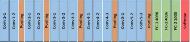
pixel is represented by a number between 0 and 255. Grey scale images are represented by a 1-D
205
array, while RGB images are represented by a 3-D array, where the colour channels (Red, Green and
206
Blue) represent the depth of the array. In the convolutional layers, different filters with smaller
207
dimensions arrays but same depth as the input image (dimensions can be 1x1xm, 3x3xm, or 5x5xm,
208
where m is the depth of the input image), are used to detect the presence of specific features or
209
patterns present in the original image. The filter slides (convolved) over the whole image starting at
210
the top left corner while computing the dot product of the pixel value in the original image with the
211
values in the filter to generate a feature map. ConvNets use pooling layers to reduce the spatial size
212
of the network by breaking down the output of the convolution layers into smaller regions were the
213
maximum value of every smaller region is taken out and the rest is dropped (max-pooling) or the
214
average of all values is computed (average-pooling) [56–58]. As a result, the number of parameters
215
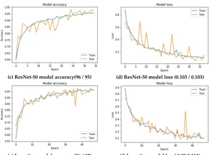
and computation required in the neural network is reduced significantly.
216
The next series of layer in ConvNets are the fully connected (FC) layers. As the name suggests,
217
it is a fully connected network of neurons (perceptrons). Every neuron in one sub-layer within the
218
FC network, has a connection with all neurons in the successive sub-layer (see Figure 1).
219
At the output layer, a classification which is based on the features extracted by the previous
220
layers is performed. Typically, for a multi-classifier neural network, a Softmax activation function is
221
considered, which outputs a probability (a number ranging from 0-1) for each of the classification
222
labels which the network is trying to predict.
223
3.2 Transfer Learning
224
According to a study by Zhu et al. [59], data dependence is one of the most challenging problems
225
in deep learning where sufficient training requires huge amounts of information in order for the
226
network to understand the patterns of data. In deep learning, both training and testing data are
227
assumed to have same distribution and same feature space. In reality, however, adequate training
228
data may exist in one domain, while a classification task is conducted on another. Moreover, if the
229
required with a newly collected training dataset. In some applications, constructing largely-enough,
231
properly-labelled datasets data can be quite challenging, particularly, when data acquisition is
232
expensive or when data annotation is the timely consuming process. This could limit the
233
development of many deep learning applications such as biomedical imaging where training data in
234
most cases is not enough to train a network. Under these circumstances, transfer learning
235
(knowledge) from one domain to another can be advantageous [32].
236
3.2.1 Mathematical Notations
237
238
Given a domain
239
𝒟 = {𝒳, 𝑃(𝑋)}, (1)
240
Then 𝒳 is the feature map, and 𝑃(X) is the probability distribution, 𝑋 = {𝑥 ,··· , 𝑥 }
241
and {𝑥 ,··· , 𝑥 } ∈ 𝒳 then the learning task 𝒯 is defined as
242
𝒯 = {𝒴, 𝑦 = 𝑃(𝑌|} (2)
243
Where 𝒴 is the set of all labels, and 𝑦 is the prediction function. The training data is
244
represented by the pairs {𝑥 , 𝑦 } where 𝑥 ∈ 𝑋, 𝑦 ∈ 𝒴.
245
246
Suppose 𝒟 denotes the source domain and 𝒟 denotes the target domain, then the source
247
domain data can be presented as:
248
𝒟 = 𝑥 , 𝑦 , ⋯ , 𝑥 , 𝑦 , (3)
249
where 𝑥 ∈ 𝒳 is the given input data, and 𝑦 ∈ 𝒴 is the corresponding label. The target
250
domain DT can also be represented in the same way:
251
252
𝒟 = 𝑥 , 𝑦 , ⋯ , 𝑥 , 𝑦 , (4)
253
where 𝑥 ∈ 𝒳 is the given input data, and 𝑦 ∈ 𝒴 is the corresponding label. In almost all
254
real-life applications, the number of data instances in the target domain is significantly less than those
255
in the source domain that is
256
257
0 ≤ 𝑛 ≪ 𝑛 (5)
258
Definition
259
For a given source domain 𝒟 and a learning task 𝒯, with target domain 𝒟 and a learning
260
task 𝒯, then transfer learning is the use of knowledge in 𝒟 and 𝒯 to improve the learning of the
261
prediction function 𝑦 in 𝒟 , given that 𝒟 ≠ 𝒟 and 𝒯 ≠ 𝒯 [60].
262
Since any domain is defined by the pair
263
264
𝒟 = {𝒳, 𝑃(𝑋)}, (6)
265
266
where 𝒳is the feature map, and 𝑃(𝑋) is the probability distribution, 𝑋 = {𝑥 ,··· , 𝑥 } ∈ 𝑋,
267
then according to the definition, if 𝒟 ≠ 𝒟
268
269
⟹ 𝒳 ≠ 𝒳 and 𝑃 (𝑋) ≠ 𝑃 (𝑋). (7)
270
Similarly, if a task is defined by
271
272
𝒯 = {𝒴, 𝑦 = 𝑃(𝑌|𝑋} (8)
where 𝒴 is the set of all labels, and 𝑦 is the prediction function, then by definition, if 𝒯 ≠ 𝒯
274
275
⟹ 𝒴 ≠ 𝒴 and, y ≠ y . (9)
276
Hence, the four possible scenarios of transfer learning are as follows:
277
1. When both target and source domains are different, that is when 𝒟 ≠ 𝒟 and their
278
feature spaces are also different, i.e. 𝒳 ≠ 𝒳 .
279
2. When the two domains are different, 𝒟 ≠ 𝒟 and their probability distribution are
280
also different, i.e. 𝑃 (𝑋) ≠ 𝑃 (𝑋), where 𝑥 ∈ 𝒳 , and 𝑃 (𝑋) ≠ 𝑃 (𝑋).
281
3. When the two domains are different, 𝒟 ≠ 𝒟 and both their learning tasks and label
282
spaces are different, that is 𝒯 ≠ 𝒯S and, 𝒴 ≠ 𝒴 , respectively.
283
4. When the target domain 𝒟 and a source domain 𝒟 are different, and their
284
conditional probability distributions are also different, that is, when y ≠ y ,
285
where
286
y = 𝑃(𝑌 |𝑋 ), (10)
287
and
288
y = 𝑃(𝑌 |𝑋 ), (11)
such that
289
𝑌 ∈ 𝒴 , 𝑌 ∈ 𝒴 .
290
If both source and target domains are the same, that is when 𝒟 = 𝒟 , the learning tasks of
291
both domains are also the same (i.e 𝒯 = 𝒯). In this scenario, the learning problem of the target
292
domain becomes a traditional machine learning approach and transfer learning is not necessary.
293
In ConvNets, transfer learning refers to using the weights of a well-trained network as an
294
initialiser for a new network. In our research, we utilized the knowledge gained by a trained
295
VGGNET on ImageNet [61] dataset which is a set that contains 14 million annotated images and
296
contains more than 20,000 categories to classify images containing mould, stain and paint
297
deterioration.
298
3.2.2 Fine-tuning
299
Fine-tuning is a way of applying transfer learning by taking a network that is already been
300
trained for some given task and then tune (or tweaks) the architecture of this network to make it
301
perform a similar task. By tweaking the architecture, we mean removing one or more layers of the
302
original model and adding new layer(s) back to perform a new (similar) task. The number of nodes
303
in the input and output layers in the original model also need to be adjusted in order to match the
304
configuration of the new model. Once the architecture of the original model has bees modified, we
305
then want to freeze the layers in the new model that came from the original model. By freezing, we
306
mean that we want the weights for these layers unchanged when the new (modified) model is being
307
re-trained on the new dataset for the new task. In this arrangement, only the weights of the new (or
308
modified) layers are updating during the re-training and the weights of the frozen layers are kept the
309
same as they were after being trained on the original task [62].
310
The amount of change in the original model, i.e. the number of layers to be replaced, primarily,
311
depends on the size of the new dataset and its similarity to the original dataset (e.g. ImageNet-like in
312
terms of the content of images and the classes, or very different, such as microscope images). When
313
the two datasets have high similarities, replacing the last layer with a new one for performing the
314
new task is sufficient. In this case, we say, transfer learning is applied as a classifier [63]. In some
315
problems, one may want to remove more than just the last single layer, and add more than just one
316
318
Figure 2. VGG-16 model. Illustration of using the VGG-16 for transfer learning. The convolution
319
layers can be used as features extractor, and the fully connected layers can be trained as a classifier.
320
3.4 Object Localisation Using Class Activation Mapping (CAM)
321
The problem of object localisation is different from image classification problem. In the latter,
322
when an algorithm looks at an image it is responsible for saying which class this image belongs to.
323
For example, our model is responsible of saying this image is a “Mould”, or a “Stain”, or a “Paint
324
deterioration” or “Normal”. In the localisation problem however, the algorithm is not only
325
responsible for determining the class of the image, it is also responsible for locating existing objects
326
in any one image, and labelling them, usually by putting a rectangular bounding box to show the
327
confidence of existence [64]. In the localisation problem, in addition to predicting the label of the
328
image, the output of the neural network also returns four numbers (x0, y0, width, and height) which
329
parameterise the bounding box of the detected object. This task requires different ConvNet
330
architecture with additional blocks of networks called Regional Proposal Networks and
Boundary-331
Box regression classifiers. The success of these methods however, rely heavily, on training datasets
332
containing lots of accurately annotated images. A detailed image annotation, e.g. manually tracing
333
an object or generating bounding boxes, however, is both expensive and often timely consuming [64].
334
A study by Zhou et al. [41] on the other hand, has shown that some layers in a ConvNet can
335
behave as object detectors without the need to provide training on the location of the object. This
336
unique ability, however, is lost when fully-connected layers are used for classification.
337
CAM is a computational-low-cost technique used with classification-trained ConvNets for
338
identifying discriminative regions in an image. In other words, CAM highlights the regions in an
339
image which are relevant to a specific class by re-using classifier layers in the ConvNet for obtaining
340
good localisation results. It was first proposed by Zhou et al. [65] to enable classification-trained
341
ConvNets to learn to perform object localisation without using any bounding box annotations.
342
Instead, the technique allows the visualisation of the predicted class scores on an input image by
343
highlighting the discriminative object parts which were detected by the neural network. In order to
344
use CAM, the network architecture must be slightly modified by adding a global average pooling
345
(GAP) after the final convolution layer. This new GAP is then used as a new feature map for the
fully-346
connected layer which generates the required (classification) output. The weights of the output layer
347
is then projected back on to the convolutional feature maps allowing a network to identify the
348
importance of the image regions. Although simple, the CAM technique uses this connectivity
349
structure to interpret the prediction decision made by the network. The CAM technique was applied
350
to our model and was able to accurately, localise defects in images as depicted in Figure 9.
351
4. Methodology
354
The aim of this research is to develop a model that classifies defects arising from dampness as
355
“mould”, “stain” or “deterioration”, should they appear in a given image, or as “normal” otherwise.
356
In this work we also examine the extent of ConvNets role in addressing challenges arising from the
357
nature of the defects under investigation and the surrounding environment. For example, according
358
to one study, mould in houses can be black, brown, green, olive-green, gray, blue, white, yellow or
359
even pink [66]. Moreover, stains and paint deterioration do not have a defined shape, size or colour
360
and their physical characteristics are heavily influenced by the surrounding environment, i.e. the
361
location (walls, ceilings, corners, etc.), the background(paint colour, wallpaper patterns, fabric, etc.)
362
and by the intensity of light under which images of these defects were taken. The irregular nature of
363
the defects imposes a big challenge when obtaining an adequate large-enough dataset to train a
364
model to classify all these cases.
365
For the purpose of this research, images containing the defect types were collected from different
366
sources. The images were then appropriately, cropped and resized to generate the dataset which was
367
used to train our model. To achieve higher accuracy, instead of training a model from scratch, we
368
adopted a transfer learning technique and used a pre-trained VGG-16 on ImageNet as our chosen
369
model to customise and initialise weights. A separate set of images, not seen by the trained model,
370
was used for validation to examine the robustness of our model. Finally, the CAM technique was
371
applied to address the localisation problem. Details of the dataset, the tuned model and final results
372
are discussed in the ensuing sections.
373
4.1 Dataset
374
Images of different resolutions and sizes were obtained from many resources, including photos
375
taken by mobile phone, a hand-held camera, and copyright-free images obtained from the internet.
376
These images were sliced into 224×224 thumbnails to increase the size of our dataset producing a total
377
number of 2622 images in our dataset. The data was labelled into four main categories: normal (image
378
containing no defects), mould, stain, and paint deterioration (which includes peeling, blistering,
379
flacking, and crazing). The total number of images used as training data was 1890: mould (534
380
images), stain (449), paint deterioration (411), and normal (496). For the validation set, 20% of the
381
training data (382 images out of the 1890 images) was randomly selected. In order to avoid overfitting
382
and for better generalisation, a broad range of image augmentations were applied to the training set,
383
including rescaling, rotation, height and width shift, horizontal and vertical flips. The remaining 732
384
images out of the 2622 were used as testing data with 183 images for each class. A sample of images
385
used is shown in Figure 3
386
Figure 3. Dataset used in this study. A sample of the dataset that was used to train our model showing
388
different mould images (first row), paint deterioration (second row), stains (third row).
389
4.2 The model
390
For our model, we applied a fine-tuning transfer learning to a VGG-16 network pre-trained on
391
ImageNet; a huge dataset of images containing more than 14 million annotated images and more
392
than 20,000 categories [60]. Our choice of using the VGG-16, is mainly because it is proven to be a
393
powerful network although having a simple architecture. This simplicity makes it easier to modify
394
for transfer learning and for the CAM technique without compromising the accuracy. Moreover,
395
VGG-16 has fewer layers (shallower) than other models such as the ResNet50 or Inception. According
396
to Kaiming et Al. [67], deeper neural networks are harder to train. Since the VGG-16 has fewer layers
397
than other networks, it makes it a better model to train on our relatively small dataset compared to
398
deeper neural networks as figure 5 shows, accuracy are close, however VGG-16 training is smoother.
399
The architecture of the VGG-16 model (illustrated in Figure 4) comprises five blocks of
400
convolutional layers with max-pooling for feature extraction. The convolutional blocks are followed
401
by three fully-connected layers and a final 1 X 1000 Softmax layer (classifier). The input to the
402
ConvNet is a 3-channel (RGB) image with a fixed size of 224 × 224. The first block consists of two
403
convolutional layers with 32 filters, each of size 3 × 3. The second, third, and forth convolution blocks
404
406
407
Figure 4. VGG-16 architecture.The VGG-16 model consists of 5 Convolution layers (in blue) each is
408
followed by a pooling layer (in orange), and 3 fully-connected layers (in green), then a final Softmax
409
classifier (in red).
410
For our model, we fine-tuned the VGG-16 model by, Firstly, freezing the early convolutional
411
layers in the VGG-16, up to the fourth block, and used them as generic feature extractor. Secondly,
412
we replaced the last 1 X 1000 Softmax layer (classifier) by a 1 X 4 classifier for classifying the 3 defects
413
and a normal class. Finally, we re-trained the newly modified model allowing only the weights of
414
block five to update during training.
415
Although different implementations of transfer learning were also examined (one by re-training
416
the whole VGG-16 model on our dataset and replacing the last (Softmax) layer by 1 x 4 classifier,
417
another implementation by freezing fewer layers and allowing weights of more layers to update
418
during training), the arrangement mentioned earlier has proven to work better.
419
4.3 Results
420
Class prediction
421
The network was trained over 50 epochs using batch of size of 32 images and a step of 250 images
422
per epoch. The final accuracy recorded at the end of the 50th epoch was 97.83% for training and
423
98.86% for the validation (Figure 5a). The final loss value was 0.0572 for training and 0.042 on the
424
validation set (Figure 5b). The plot of accuracy in Figure 5.a, also shows that the model has trained
425
well although the trend for accuracy on both validation, and training datasets is still rising for the
426
last few epochs. It also shows that all models have not over-learned the training dataset, showing
427
similar learning skills on both datasets despite the spiky nature of the validation curve. Similar
428
learning pattern can also be observed from Figure 5b as both datasets are still converging for the last
429
few epochs with a comparable performance on both training and validation datasets. Figure 5 also
430
shows that all models had no overfitting problem during the training as the validation curve is
431
converging adjacently to training curve and has not diverted away from the training curve.
432
(c) ResNet-50 model accuracy(96 / 95) (d) ResNet-50 model loss (0.103 / 0.103)
(e) Inception model accuracy (96 / 95) (f) Inception model loss( 0.09 0.144)
433
Figure 5. Comparative models accuracy and loss diagram.In sub-figure a) the VGG-16 model final
434
accuracy is 97.83% for training and 98.86% for the validation. In sub-figure b) the final loss is 0.0572
435
for training and 0.042 on the validation set. In sub-figure c) the ReseNet-50 model final accuracy is
436
96.23% for training and 95.61% for the validation. In sub-figure d) the final loss is 0.103 for training
437
and 0.102 on the validation set. In sub-figure e) the Inception model final accuracy is 96.77% for
438
training and 95.42% for the validation. In sub-figure f) the final loss is 0.109 for training and 0.144 on
439
the validation set.
440
To test the robustness of our model, we performed a prediction test on 732 non-used images
441
dedicated for evaluating our model. The accuracy after completing the test was high and reached
442
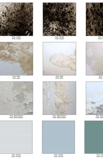
87.50%. A sample example of correct classification of different types of defects is shown in Figure 6.
443
In this figure, representative images show the accurate classification of our model to the four classes:
444
in the first row, mould prediction (n= 167 out of 183), in the second row stain prediction, (n= 145 out
445
of 183), in the third row deterioration prediction (n=157 out of 183) and in the fourth row the
446
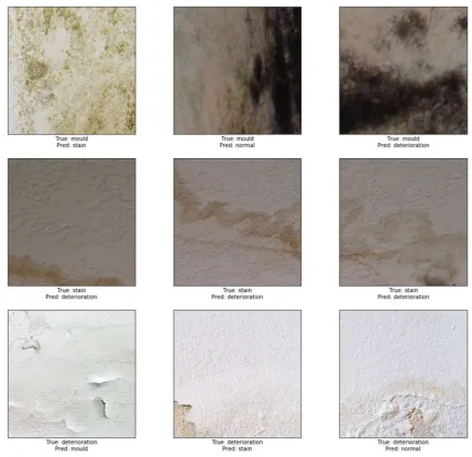
prediction of normal class (n= 183 out of 183). An example of miss-classified defects is shown in
447
Figure 7. The representative images in this figure show failure of the model to correctly predict the
448
correct class. 38 images containing stains were miss-classified; 31 as paint deterioration and 6 as
449
mould and 1 as normal. 26 images containing paint deterioration were miss-classified; 13 as mould
450
and 13 as stain. 16 images containing mould were miss-classified; 4 as paint deterioration and 12 as
451
stain. The results in this figure illustrates an example where our model failed to identify the correct
452
class of the damage caused by the damp. The false predictions for images by modern neural networks
453
have been studied by many researcher [68–72]. According to Nguyen et Al. [68], although modern
454
deep neural network achieved state-of-the-art performance and are able to classify objects in images
455
with near-human-level accuracy, a slight change in an image, invisible to human eye can easily fool
456
the neural network and cause it to miss-label the image. Guo et al. argues that this is primarily due
457
to the fact that neural networks are overconfident in their predictions and often outputs highly
458
relationship between the accuracy of neural network and the predictions scores (confidence).
460
According to the authors, a network with a confidence rate equal to accuracy rate is a calibrated neural
461
network. However, they concluded that, although the capacity of neural networks has increased
462
significantly in the past years, the increasing depth of modern neural networks negatively affects
463
model calibration [70].
464
465
Figure 6. Correct classification of mould, stain and deterioration.
466
Figure 7. Example of miss-classification.
468
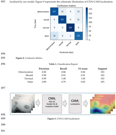
Our model, has performed very well on detecting images with mould with success rate of
469
around 91%. The largest number of miss-classified defects occur in the stain and deterioration classes,
470
with approximately 85% success rate in classifying stain and also 80% success rate in classifying paint
471
deterioration (Figure 8). In Table 1, it can be seen that the overall precision of the model ranges
472
between 82% for detecting deterioration, 84% for mould, and 89% for stain. The recall analysis show
473
similar results, with 82% for detecting deterioration, 90% for mould, 99% for normal, and 89% for
474
stain. Note that the precision which is the ability of the classifier to label positive classes as positive
475
is the ratio tp / (tp + fp) where tp is the number of true positives and fp the number of false positives.
476
The recall quantifies the ability of the classifier to find all the positive samples, that is the
477
ratio tp / (tp + fn) where fn is number of false negatives. F1 Score is the weighted average of precision
478
and recall, that is F1 Score = 2*(Recall * Precision) / (Recall + Precision).
479
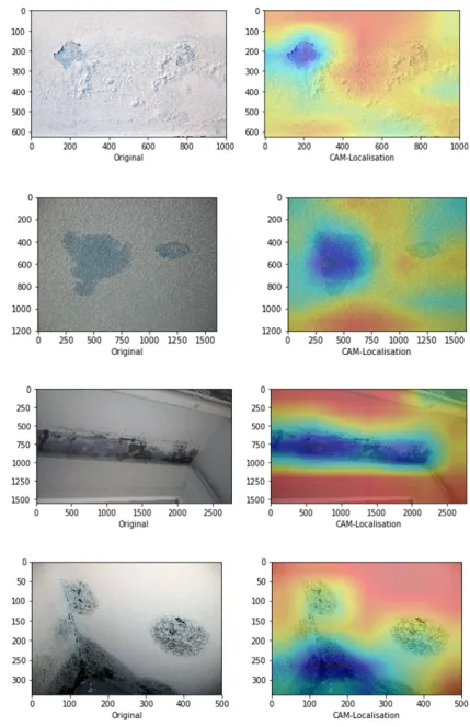
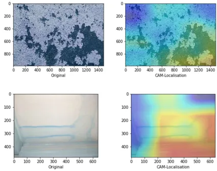
Defect localisation using CAM
480
Following the high accuracy in detecting the three classes we then, asked the question: can our
481
model detect the actual localisation of these classes? To do so, we integrated the CAM [41] with our
482
network. The CAM is a technique that uses the gradient of an object under consideration entering the
483
final convolutional layer of the ConvNet to produces a coarse localisation map which highlights the
484
most significant regions in the image for predicting the class of this image. It can be seen from the
485
CAM method: in first row sample of images containing paint deterioration, in second row a sample
487
of images containing stains, and in third and fourth rows samples of images containing mould that,
488
our model has accurately allocated the defect in each image with high precision. In few cases,
489
however, incorrect localisation was obtained, for example the images in Figure 11 showing some
490
defect incorrectly located by our model. Although the first image contains paint deterioration spread
491
over large areas of the image and the second image contains a large stain, both defects were
miss-492
localised by our model. Figure 9 represents the schematic illustration of CNN-CAM localisation.
493
494
Figure 8. Confusion Matrix.
495
Table 1. Classification Report.
496
Precision Recall F1-score Support
Deterioration 0.82 0.86 0.84 183
Mould 0.90 0.91 0.91 183
Normal 0.99 1.00 1.00 183
Stain 0.89 0.79 0.82 183
497
498
Figure 9. CNN-CAM localisation
499
500
501
502
505
Figure 11. Incorrect localisation.
506
5. Discussion and Conclusions
507
The work is concerned with the development of a deep learning-based method for the
508
automated detection and localisation of key building defects from given images. This research is part
509
of work on condition assessment of built assets. The developed approach involves classification of
510
images into four categories: three categories of building defects caused by dampness namely: mould,
511
stain and paint deterioration which includes peeling, blistering, flacking, and crazing and of these
512
defects and a fourth category “Normal” when no defects is present.
513
For our classification problem, we applied a fine-tuning transfer learning to a VGG-16 network
514
pre-trained on ImageNet. A total of 2622 224x 224 images were used as our dataset. Out of the 2622
515
images, a total 1890 images used for training data: mould (534 images), stain (449), paint deterioration
516
(411) and normal (496). In order to obtain sufficient robustness, we applied different augmentation
517
techniques to generate larger dataset. For the validation set, a 20% of the training data (382 images)
518
was randomly chosen. After 50 epochs, the network recorded an accuracy of 97.83% with 0.0572 loss
519
on the training set and 98.86% with 0.042 loss on the validation. The robustness of our network was
520
evaluated on a separate set of 732 images, 183 images for each class. The evaluation test showed a
521
consistent overall accuracy of 87.50% and %90 of images containing mould correctly classified, 82%
522
for images containing deterioration, 89% for images containing stain and 99% for normal images. To
523
address the localisation problem, we integrated the CAM technique which was able to locate defects
524
with high precision. The overall performance of the proposed network has shown high reliability and
525
robustness in classifying and localising defects. The main challenge during this work was the
526
To overcome this obstacle, we used image augmentation techniques to generate synthetic data for a
528
largely enough dataset to train our model.
529
The benefit of our approach, lays in the fact that, whilst similar research such as the one by Cha
530
et al.[48] and others [26,28,59,73], focus only on detecting cracks on concrete surfaces which is a
531
simple binary classification problem, we offer a method to build a powerful model that can accurately
532
detect and classify multi-class defects given a relatively very small datasets. Whilst cracks in
533
constructions have been widely studies and supported by large dedicated datasets such as [74] and
534
[75], our work, describe herewith in, offers a roadmap for researcher in condition assessment of built
535
assets to study other types of equally important defects which have not been addressed sufficiently.
536
For the future works, the challenges and limitation that we were facing this in paper will be
537
addressed. The presented paper had to set a number of limitations, i.e., firstly, multiple types of the
538
defects are not considered at once. This means that the images considered by the model belonged to
539
only one category. Secondly, only the images with visible defects are considered. Thirdly,
540
consideration of the extreme lighting and orientation, e.g., low lighting, too bright images, are not
541
included in this study. In the future works, these limitations will be considered to be able to get closer
542
to the concept of a fully automated detection. Through fully satisfying these challenges and
543
limitations, our present work will be evolved into a software application to perform real-time
544
detection of defects using vision sensors including drones. The work will also be extended to cover
545
other models that can detect other defects in construction such as cracks, structural movements,
546
spalling and corrosion. Our long-term vision includes plans to create a large, open source database
547
of different building and construction defects which will support world-wide research on condition
548
assessment of built assets.
549
References
550
1. Mohseni, H.; Setunge, S.; Zhang, G. M.; Wakefield, R. In Condition monitoring and condition aggregation
551
for optimised decision making in management of buildings, Applied Mechanics and Materials, 2013; Trans
552
Tech Publ: 2013; pp 1719-1725.
553
2. Agdas, D.; Rice, J. A.; Martinez, J. R.; Lasa, I. R., Comparison of visual inspection and structural-health
554
monitoring as bridge condition assessment methods. Journal of Performance of Constructed Facilities 2015,
555
30, (3), 04015049.
556
3. Shamshirband, S.; Mosavi, A.; Rabczuk, T., Particle swarm optimization model to predict scour depth
557
around bridge pier. arXiv preprint arXiv:1906.08863 2019.
558
4. Zhang, Y.; Anderson, N.; Bland, S.; Nutt, S.; Jursich, G.; Joshi, S., All-printed strain sensors: Building blocks
559
of the aircraft structural health monitoring system. Sensors and Actuators A: Physical 2017, 253, 165-172.
560
5. Noel, A. B.; Abdaoui, A.; Elfouly, T.; Ahmed, M. H.; Badawy, A.; Shehata, M. S., Structural health monitoring
561
using wireless sensor networks: A comprehensive survey. IEEE Communications Surveys & Tutorials 2017,
562
19, (3), 1403-1423.
563
6. Kong, Q.; Allen, R. M.; Kohler, M. D.; Heaton, T. H.; Bunn, J., Structural health monitoring of buildings
564
using smartphone sensors. Seismological Research Letters 2018, 89, (2A), 594-602.
565
7. Song, G.; Wang, C.; Wang, B., Structural health monitoring (SHM) of civil structures. In Multidisciplinary
566
DigitalPublishing Institute: 2017.
567
8. Annamdas, V. G. M.; Bhalla, S.; Soh, C. K., Applications of structural health monitoring technology in Asia.
568
Structural Health Monitoring 2017, 16, (3), 324-346.
569
9. Lorenzoni, F.; Casarin, F.; Caldon, M.; Islami, K.; Modena, C., Uncertainty quantification in structural health
570
monitoring: Applications on cultural heritage buildings. Mechanical Systems and Signal Processing 2016,
571
10. Oh, B. K.; Kim, K. J.; Kim, Y.; Park, H. S.; Adeli, H., Evolutionary learning based sustainable strain sensing
573
model for structural health monitoring of high-rise buildings. Applied Soft Computing 2017, 58, 576-585.
574
11. Mita, A. In Gap between technically accurate information and socially appropriate information for
575
structural health monitoring system installed into tall buildings, Health Monitoring of Structural and
576
Biological Systems 2016, 2016; International Society for Optics and Photonics: 2016; p 98050E.
577
12. Mimura, T.; Mita, A., Automatic estimation of natural frequencies and damping ratios of building
578
structures. Procedia Engineering 2017, 188, 163-169.
579
13. Zhang, F. L.; Yang, Y. P.; Xiong, H. B.; Yang, J. H.; Yu, Z., Structural health monitoring of a 250-m super-tall
580
building and operational modal analysis using the fast Bayesian FFT method. Structural Control and Health
581
Monitoring 2019, e2383.
582
14. Davoudi, R.; Miller, G. R.; Kutz, J. N., Structural load estimation using machine vision and surface crack
583
patterns for shear-critical RC beams and slabs. Journal of Computing in Civil Engineering 2018, 32, (4),
584
04018024.
585
15. Hoang, N. D., Image Processing-Based Recognition of Wall Defects Using Machine Learning Approaches
586
and Steerable Filters. Comput. Intell. Neurosci. 2018, 2018.
587
16. Jo, J.; Jadidi, Z.; Stantic, B., A drone-based building inspection system using software-agents. In Studies in
588
Computational Intelligence, Springer Verlag: 2017; Vol. 737, pp 115-121.
589
17. Pahlberg, T.; Thurley, M.; Popovic, D.; Hagman, O., Crack detection in oak flooring lamellae using
590
ultrasound-excited thermography. Infrared Phys Technol 2018, 88, 57-69.
591
18. Pragalath, H.; Seshathiri, S.; Rathod, H.; Esakki, B.; Gupta, R., Deterioration assessment of infrastructure
592
using fuzzy logic and image processing algorithm. Journal of Performance of Constructed Facilities 2018,
593
32, (2), 04018009.
594
19. Valero, E.; Forster, A.; Bosché, F.; Hyslop, E.; Wilson, L.; Turmel, A., Automated defect detection and
595
classification in ashlar masonry walls using machine learning. Autom Constr 2019, 106.
596
20. Valero, E.; Forster, A.; Bosché, F.; Renier, C.; Hyslop, E.; Wilson, L. In High Level-of-Detail BIM and Machine
597
Learning for Automated Masonry Wall Defect Surveying, ISARC. Proceedings of the International
598
Symposium on Automation and Robotics in Construction, 2018; IAARC Publications: 2018; pp 1-8.
599
21. Lee, B.J.; Lee, H. “David” Position-invariant neural network for digital pavement crack analysis.
Comput.-600
Aided Civ. Infrastruct. Eng. 2004, 19, 105–118.
601
22. Koch, C.; Brilakis, I. Pothole detection in asphalt pavement images. Adv. Eng. Inform. 2011, 25, 507–515.
602
23. Cord, A.; Chambon, S. Automatic road defect detection by textural pattern recognition based on AdaBoost.
603
Comput.-Aided Civ. Infrastruct. Eng. 2012, 27, 244–259.
604
24. Jahanshahi, M.R.; Jazizadeh, F.; Masri, S.F.; Becerik-Gerber, B. Unsupervised approach for autonomous
605
pavement-defect detection and quantification using an inexpensive depth sensor. J. Comput. Civ. Eng. 2012,
606
27, 743–754.
607
25. Radopoulou, S.C.; Brilakis, I. Automated detection of multiple pavement defects. J. Comput. Civ. Eng. 2016,
608
31, 04016057.
609
26. Abdel-Qader, I.; Abudayyeh, O.; Kelly, M.E. Analysis of edge-detection techniques for crack identification
610
in bridges. J. Comput. Civ. Eng. 2003, 17, 255–263.
611
27. Duran, O.; Althoefer, K.; Seneviratne, L.D. State of the art in sensor technologies for sewer inspection. IEEE
612
Sens. J. 2002, 2, 73–81.
613
28. Sinha, S.K.; Fieguth, P.W. Automated detection of cracks in buried concrete pipe images. Autom. Constr.
614
29. Sinha, S.K.; Fieguth, P.W. Neuro-fuzzy network for the classification of buried pipe defects. Autom. Constr.
616
2006, 15, 73–83.
617
30. Guo, W.; Soibelman, L.; Garrett, J.H. Visual Pattern Recognition Supporting Defect Reporting and Condition
618
Assessment of Wastewater Collection Systems. J. Comput. Civ. Eng. 2009, 23, 160–169.
619
31. Huang, G.; Liu, Z.; Weinberger, K.Q. Densely Connected Convolutional Networks. CoRR 2016,
620
abs/1608.06993.
621
32. German, S.; Brilakis, I.; DesRoches, R. Rapid entropy-based detection and properties measurement of
622
concrete spalling with machine vision for post-earthquake safety assessments. Adv. Eng. Inform. 2012, 26,
623
846–858.
624
33. Ji, M.; Liu, L.; Buchroithner, M. Identifying Collapsed Buildings Using Post-Earthquake Satellite Imagery
625
and Convolutional Neural Networks: A Case Study of the 2010 Haiti Earthquake. Remote Sens. 2018, 10.
626
34. Organisation (ISO), I.S. ISO 19208:2016- Framework for specifying performance in buildings; ISO, 2016;
627
35. Limited, C.S. Defects in Buildings: Symptoms, Investigation, Diagnosis and Cure; Stationery Office, 2001;
628
36. Seeley, I.H. Building maintenance; Macmillan International Higher Education, 1987;
629
37. Richardson, B. Defects and Deterioration in Buildings: A Practical Guide to the Science and Technology of
630
Material Failure; Routledge, 2002;
631
38. Wood, B.J. Building maintenance; John Wiley & Sons, 2009;
632
39. Riley, M.; Cotgrave, A. Construction technology 3: The technology of refurbishment and maintenance;
633
Macmillan International Higher Education, 2011;
634
40. Simonyan, K.; Zisserman, A. Very deep convolutional networks for large-scale image recognition. ArXiv
635
Prepr. ArXiv14091556 2014.
636
41. Zhou, B.; Khosla, A.; Lapedriza, A.; Oliva, A.; Torralba, A. Learning deep features for discriminative
637
localization. In Proceedings of the Proceedings of the IEEE conference on computer vision and pattern
638
recognition; 2016; pp. 2921–2929.
639
42. Trotman, P.M.; Harrison, H. Understanding dampness; BREbookshop, 2004;
640
43. Burkinshaw, R.; Parrett, M. Diagnosing damp; RICS books, 2003;
641
44. Thomas, A.R. Treatment of damp in old buildings; Technical pamphlet 8, Society for the protection of
642
ancient buildings, Eyre & Spottiswoode Ltd, 1986;
643
45. Lourenço, P.B.; Luso, E.; Almeida, M.G. Defects and moisture problems in buildings from historical city
644
centres: a case study in Portugal. Build. Environ. 2006, 41, 223–234.
645
46. Bakri, N.N.O.; Mydin, M.A.O. General building defects: causes, symptoms and remedial work. Eur. J.
646
Technol. Des. 2014, 4–17.
647
47. Wang, W.; Wu, B.; Yang, S.; Wang, Z. Road Damage Detection and Classification with Faster R-CNN. In
648
Proceedings of the 2018 IEEE International Conference on Big Data (Big Data); IEEE, 2018; pp. 5220–5223.
649
48. Cha, Y.-J.; Choi, W.; Suh, G.; Mahmoudkhani, S.; Büyüköztürk, O. Autonomous structural visual inspection
650
using region-based deep learning for detecting multiple damage types. Comput.-Aided Civ. Infrastruct.
651
Eng. 2018, 33, 731–747.
652
49. Roth, H.; Farag, A.; Lu, L.; B. Turkbey, E.; Summers, R. Deep convolutional networks for pancreas
653
segmentation in CT imaging. 2015, 9413.
654
50. Fukushima, K. A neural network for visual pattern recognition. Computer 1988, 65–75.
655
51. Rawat, W.; Wang, Z. Deep convolutional neural networks for image classification: A comprehensive review.
656
52. A “Brief” History of Neural Nets and Deep Learning Available online:
/writing/ai/a-brief-history-of-neural-658
nets-and-deep-learning/ (accessed on Jun 27, 2019).
659
53. Stathakis, D. How many hidden layers and nodes? Int. J. Remote Sens. 2009, 30, 2133–2147.
660
54. Smithson, S.C.; Yang, G.; Gross, W.J.; Meyer, B.H. Neural Networks Designing Neural Networks:
Multi-661
Objective Hyper-Parameter Optimization. ArXiv161102120 Cs 2016.
662
55. Heaton, J. Introduction to Neural Networks with Java; Heaton Research, Inc., 2008; ISBN
978-1-60439-008-663
7.
664
56. Lee, C.-Y.; Gallagher, P.W.; Tu, Z. Generalizing Pooling Functions in Convolutional Neural Networks:
665
Mixed, Gated, and Tree. 9.
666
57. Giusti, A.; Cireşan, D.C.; Masci, J.; Gambardella, L.M.; Schmidhuber, J. Fast image scanning with deep
max-667
pooling convolutional neural networks. In Proceedings of the 2013 IEEE International Conference on Image
668
Processing; 2013; pp. 4034–4038.
669
58. Yu, D.; Wang, H.; Chen, P.; Wei, Z. Mixed Pooling for Convolutional Neural Networks. In Proceedings of
670
the Rough Sets and Knowledge Technology; Miao, D., Pedrycz, W., Ślȩzak, D., Peters, G., Hu, Q., Wang, R.,
671
Eds.; Springer International Publishing, 2014; pp. 364–375.
672
59. Visual retrieval of concrete crack properties for automated post-earthquake structural safety evaluation.
673
Autom. Constr. 2011, 20, 874–883.
674
60. Pan, S.J.; Yang, Q. A Survey on Transfer Learning. IEEE Trans. Knowl. Data Eng. 2010, 22, 1345–1359.
675
61. Deng, J.; Dong, W.; Socher, R.; Li, L.-J.; Kai Li; Li Fei-Fei ImageNet: A large-scale hierarchical image
676
database. In Proceedings of the 2009 IEEE Conference on Computer Vision and Pattern Recognition; IEEE:
677
Miami, FL, 2009; pp. 248–255.
678
62. Ge, W.; Yu, Y. Borrowing Treasures from the Wealthy: Deep Transfer Learning through Selective Joint
Fine-679
tuning. ArXiv170208690 Cs Stat 2017.
680
63. Hu, J.; Lu, J.; Tan, Y.-P. Deep Transfer Metric Learning.; 2015; pp. 325–333.
681
64. Zhao, Z.-Q.; Zheng, P.; Xu, S.; Wu, X. Object Detection with Deep Learning: A Review. ArXiv180705511 Cs
682
2018.
683
65. Zhou, B.; Khosla, A.; Lapedriza, A.; Oliva, A.; Torralba, A. Object Detectors Emerge in Deep Scene CNNs.
684
ArXiv14126856 Cs 2014.
685
66. Guide to Mold Colors and What They Mean Available online:
http://www.safebee.com/home/guide-to-686
mold-colors-what-they-mean (accessed on Jun 19, 2019).
687
67. He, K.; Zhang, X.; Ren, S.; Sun, J. Deep Residual Learning for Image Recognition. CoRR 2015, abs/1512.03385.
688
68. Nguyen, A.; Yosinski, J.; Clune, J. Deep Neural Networks are Easily Fooled: High Confidence Predictions
689
for Unrecognizable Images. ArXiv14121897 Cs 2014.
690
69. Lee, K.; Lee, H.; Lee, K.; Shin, J. Training Confidence-calibrated Classifiers for Detecting Out-of-Distribution
691
Samples. ArXiv171109325 Cs Stat 2017.
692
70. Guo, C.; Pleiss, G.; Sun, Y.; Weinberger, K.Q. On Calibration of Modern Neural Networks. ArXiv170604599
693
Cs 2017.
694
71. Amodei, D.; Olah, C.; Steinhardt, J.; Christiano, P.; Schulman, J.; Mané, D. Concrete Problems in AI Safety.
695
ArXiv160606565 Cs 2016.
696
72. DeVries, T.; Taylor, G.W. Learning Confidence for Out-of-Distribution Detection in Neural Networks.
697
ArXiv180204865 Cs Stat 2018.
698
73. Cha, Y.-J.; Choi, W.; Büyüköztürk, O. Deep learning-based crack damage detection using convolutional
699
74. Özgenel, Ç.F. Concrete Crack Images for Classification. 2018, 1.
701
75. Maguire, M.; Dorafshan, S.; Thomas, R. SDNET2018: A concrete crack image dataset for machine learning
702
applications. Browse Datasets 2018.