with Extreme Pruning
Yoshinori Aono1, Phong Q. Nguyen2,3, Takenobu Seito4, and Junji Shikata5 1 National Institute of Information and Communications Technology, Japan
2 Inria Paris, France
3 CNRS, JFLI, University of Tokyo, Japan 4 Bank of Japan?, Japan
5 Yokohama National University, Japan
Abstract. At Eurocrypt ’10, Gama, Nguyen and Regev introduced lat-tice enumeration with extreme pruning: this algorithm is implemented in state-of-the-art lattice reduction software and used in challenge records. They showed that extreme pruning provided an exponential speed-up over full enumeration. However, no limit on its efficiency was known, which was problematic for long-term security estimates of lattice-based cryptosystems. We prove the first lower bounds on lattice enumeration with extreme pruning: if the success probability is lower bounded, we can lower bound the global running time taken by extreme pruning. Our re-sults are based on geometric properties of cylinder intersections and some form of isoperimetry. We discuss their impact on lattice security estimates.
1
Introduction
Among all the candidates submitted in 2017 to the NIST standardization of post-quantum cryptography, the majority are based on hard lattice problems, such as LWE and NTRU problems. Unfortunately, security estimates for lattice problems are known to be difficult: many different assessments exist in the re-search literature, which is reflected in the wide range of security estimates in NIST submissions (see [2]), depending on the model used. One reason is that the performance of lattice algorithms depends on many parameters: we do not know how to select these parameters optimally, and we do not know how far from optimal are current parameter selections. The most sensitive issue is the evaluation of the cost of a subroutine to find shortest or nearly shortest lattice vectors in certain dimensions (typically the blocksize of blockwise reduction al-gorithms). In state-of-the-art lattice reduction software [11,7,9], this subroutine is implemented by lattice enumeration with extreme pruning, introduced at Eurocrypt ’10 by Gama, Nguyen and Regev [16] as a generalization of pruning methods introduced by Schnorret al[34,35] in the 90s. Yet, most lattice-based
NIST submissions chose their parameters based on the assumption that siev-ing [1,28,22,20,8] (rather than enumeration) is the most efficient algorithm for this subroutine. This choice goes back to the analysis of NewHope [3, Sect. 6], which states that sieving is more efficient than enumeration in dimension≥250 for both classical and quantum computers, based on a lower bound on the cost of sieving (ignoring subexponential terms) and an upper bound on the cost of of enumeration (either [11, Table 4] or [10, Table 5.2]). In dimensions around 140−150, this upper bound is very close to actual running times for solving the largest record SVP challenges [32], which does not leave much margin for future progress; and for dimensions≥250, a numerical extrapolation has been used, which is also debatable.
It would be more consistent to compare the sieving lower bound by a lower bound on lattice enumeration with extreme pruning. Unfortunately, no such lower bound is known: the performances of extreme pruning strongly depends on the choice of bounding function, and it is unknown how good can be such a function. There is only a partial lower bound on the cost of extreme pruning in [11], assuming that the choice of step bounding function analyzed in [16] is optimal. And this partial lower bound is much lower than the upper bound given in [11,10].
Our results. We study the limitations of lattice enumeration with extreme prun-ing. We prove the first lower bound on the cost of extreme pruning, given a lower bound on the global success probability. This is done by studying the case of a single enumeration with cylinder pruning, and generalizing it to the extreme pruning case of multiple enumerations, possibly infinitely many. Our results are based on geometric properties of cylinder intersections and a prob-abilistic form of isoperimetry: usually, isoperimetry refers to a geometric in-equality involving the surface area of a set and its volume.
Our lower bounds are easy to compute and appear to be reasonably tight in practice, at least in the single enumeration case: we introduce a cross-entropy-based method which experimentally finds upper bounds somewhat close to our lower bounds.
Reduced Basis Model
Simulated HKZ basis Rankin basis
Computing
Model
Classical
Quantum
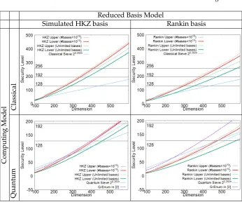
Fig. 1.Upper/lower bounds on the classical/quantum cost of enumeration with cylin-der pruning, using strongly-reduced basis models. See Sect. 5 for the exact meaning of these curves: the lower bounds correspond to (16) and (17) and the upper bounds are found by the algorithm in Sect. 4. For comparison, we also displayed several curves from [2]: 20.292nand 20.265nas the simplified classical/quantum complexity of sieve al-gorithms, and the numerical extrapolation of enumeration cost of [17, (2)].
Technical overview. Enumeration is the simplest algorithm to solve hard lattice problems: it outputsL∩B, given a latticeLand ann-dimensional ballB⊆Rn.
Cylinder pruning uses the intersectionSofncylinders defined by a lattice basis and a bounding function f: by using different lattice basesB, one obtains different setsS. The running time and the success probability of cylinder prun-ing depend on the quality of the basis, and the boundprun-ing function f. But when one uses different bases, these bases typically have approximately the same quality, which allows to focus on f, which determines the radii ofS.
The probability of success of cylinder pruning is related to the volume ofS, whereas its cost is related to the volumes of the ’canonical’ projections ofS. We show that if the success probability is lower bounded, that is, ifSis sufficiently big (with respect to its volume, or its Gaussian measure for the case of solving LWE), then the function f definingScan be lower bounded: as a special case, ifSoccupies a large fraction of the ball, f is lower bounded by essentially the linear pruning function of [16]. This immediately gives lower bounds on the volumes of the projections ofS, but we significantly improve these direct lower bounds using the following basic form of isoperimetry: for certain distributions such as the Gaussian distribution, among all Borel sets of a given volume, the ball centered at the origin has the largest probability. The extreme pruning case is obtained by a refinement of isoperimetry over finitely many sets: it is some-what surprising that we obtain a lower bound even in the extreme case where we allow infinitely many setsS.
All our lower bounds are easy to compute. To evaluate their tightness, we introduce a method based on cross-entropy to compute good upper bounds in practice, i.e., good choices of f. This is based on earlier work by Chen [10].
Open problem. Our lower bounds are specific to cylinder pruning [16]. It would be interesting to obtain tight lower bounds for discrete pruning [5].
Roadmap. In Section 2, we introduce background and notation on lattices, enu-meration and its cost estimations. Section 3 presents our lower bounds as geo-metric properties of cylinder intersections. Section 4 shows how to obtain good upper bounds in practice, by finding nice cylinder intersections using cross-entropy. Finally, in Section 5, we evaluate the tightness of our lower bounds and discuss security estimates for the hardness of finding nearly shortest lattice vectors. The appendix includes proofs of technical results. The full version of this paper on eprint also includes sage scripts to compute our lower bounds.
2
Background
2.1 Notation
Throughout the paper, we use row representations of matrices. The Euclidean norm of a vectorv ∈Rnis denotedkvk. The ’canonical’ projection ofu ∈Rn
Measures. We denote by vol the standard Lebesgue measure overRn. We de-note byρn,σthe centered Gaussian measure of varianceσ2, whose pdf overRn
is
(2πσ2)−n/2e−kxk2/(2σ2).
The standard Gaussian measure isρn =ρn,1.
Balls. We denote by Balln(R)then-dimensional zero-centered ball of radiusR.
LetVn(R) =vol(Balln(R)). Letu= (u1, . . . ,un)be a point chosen uniformly at
random from the unit sphereSn−1,e.g. ui =xi/
q ∑n
j=1x2j, wherex1, . . . ,xn are
independent, normally distributed random variables with mean 0 and variance
1. Thenkτk(u)k2= ∑
k i=1x2i ∑k
i=1x2i+∑ni=k+1x2i
= XX+Y, whereXandYhave distributions
Gamma(k/2,θ= 2)and Gamma((n−k)/2,θ=2)respectively. Here, we use
the scale parametrization to represent Gamma distributions. Hence,kτk(u)k2
has distribution Beta(k/2,(n−k)/2). In particular,kτn−2(u)k2has distribution Beta(n/2−1, 1), whose pdf isx(n/2)−2/B(n/2−1, 1) = (n/2−1)x(n/2)−2. It follows that the truncation τn−2(u) is uniformly distributed over Balln−2(1), which allows to transfer our results to random points in balls.
Recall that the cumulative distribution function of the Beta(a,b)distribution is the regularized incomplete beta functionIx(a,b)defined as:
Ix(a,b) = 1 B(a,b)
Z x
0 u
a−1(1−u)b−1du, (1)
whereB(a,b) = ΓΓ((aa)+Γ(bb))denotes the beta function. We have the following ele-mentary bounds (by integrating by parts):
xa(1−x)b−1
aB(a,b) ≤Ix(a,b) ∀a>0,b≥1, 0≤x≤1 (2)
Ix(a,b)≤ x a
a·B(a,b) ∀a>0,b≥1, 0≤x≤1 (3)
Forz ∈ [0, 1]anda,b > 0,I−1
z (a,b) +I1−−1z(b,a) =1 which is immediate from
the relationIx(a,b) +I1−x(b,a) =1.
Finally,P(s,x) = Rx
0 ts−1e−tdt/Γ(s)is the regularized incomplete gamma function.
Lattices. Alattice Lis a discrete subgroup ofRm, or equivalently the set
L(b1, . . . ,bn) = {∑ni=1xibi : xi∈Z}of all integer combinations ofnlinearly
independent vectorsb1, . . . ,bn ∈Rm. Suchbi’s form abasisofL. All the bases
ofLhave the same numbernof elements, called the dimension or rank ofL, and the samen-dimensional volume of the parallelepiped{∑n
i=1aibi : ai ∈[0, 1)}
denote it by covol(L). The latticeL is said to befull-rank ifn = m. The most famous lattice problem is theshortest vector problem(SVP), which asks to find a non-zero lattice vector of minimal Euclidean norm. Theclosest vector problem (CVP) asks to find a lattice vector closest to a target vector.
Orthogonalization. For a basisB= (b1, . . . ,bn)of a latticeLandi∈ {1, . . . ,n},
we denote byπi the orthogonal projection on span(b1, . . . ,bi−1)⊥. The Gram-Schmidt orthogonalizationof the basisB is defined as the sequence of orthogo-nal vectors B? = (b?1, . . . ,b?n), where b?i := πi(bi). We can write each bi as
b?i +∑ij−=11µi,jb?j for some uniqueµi,1, . . . ,µi,i−1 ∈ R. Thus, we may represent theµi,j’s by a lower-triangular matrixµwith unit diagonal. The projection of a
lattice may not be a lattice, butπi(L)is ann+1−idimensional lattice
gener-ated byπi(bi), . . . ,πi(bn), with covol(πi(L)) =∏nj=i
b?j
.
The Gaussian Heuristic. For a full-rank latticeLinRnand a measurable setC⊂ Rn, the Gaussian heuristic estimates the number of lattice points inside ofC
to be approximately vol(C)/vol(L). Accordingly, we would expect thatλ1(L) might be close to GH(L) = Vn(1)−1/nvol(L)1/n, which holds for a random
latticeL.
Cylinders. The performances of cylinder pruning are directly related to the fol-lowing bodies. Define the (k-dimensional) cylinder-intersection of radiiR1 ≤ · · · ≤Rkas the set
CR1,...,Rk =
(
(x1, . . . ,xk)∈Rk, ∀j≤k, j
∑
`=1
x2` ≤R2j )
⊆Ballk(Rk).
Gama et al. [16] showed how to efficiently compute tight lower and upper bounds for vol(CR1,...,Rk), thanks to the Dirichlet distribution and special in-tegrals.
2.2 Enumeration with Cylinder Pruning
To simplify notations, we assume that we focus on the SVP setting,i.e.to find short lattice vectors, rather than the more general CVP setting. LetLbe a full-rank lattice in Rn. Given a basis B = (b
1, . . . ,bn)of Land a radius R > 0,
Enumeration [29,18,15] outputsL∩SwhereS=Balln(R)by a depth-first tree
search: by comparing all the norms of the vectors obtained, one extracts a short-est non-zero lattice vector.
We follow the general pruning framework of [5], which replacesSby a sub-set ofSdepending onB. Given a functionf :{1, . . . ,n} →[0, 1], Gamaet al.[16] introduced the following set to generalize the pruned enumeration of [34,35]:
where theπiis the projection over span(b1, . . . ,bi−1)⊥. The setPf(B,R)should
be viewed as a random variable. Note thatPf(B,R) ⊆ Balln(R)and ifgis the
constant function equal to 1, thenPg(B,R) =Balln(R).
Gamaet al.[16] noticed that the basic enumeration algorithm can actually computeL∩Pf(B,R)instead ofL∩Balln(R), just by changing its parameters.
We callcylinder pruningthis form of pruned enumeration, becausePf(B,R)is
an intersection of cylinders, since each equationkπn+1−i(x)k ≤ f(i)Rdefines a
cylinder. Cylinder pruning was historically introduced in the SVP setting, but its adaptation to CVP is straightforward, as was shown by Liu and Nguyen [21].
Complexity of Enumeration. The advantage is that for suitable choices of f, enu-meratingL∩Pf(B,R)is much cheaper than enumeratingL∩Balln(R): indeed,
[16] shows that cylinder pruning runs in∑n
k=1Nkpoly-time operations, where Nk is the number of points of πn+1−k(L∩Pf(B,R)): this is because Nk is
ex-actly the number of nodes at depthn−k+1 of the enumeration tree which is searched by cylinder pruning. By the Gaussian heuristic, we have heuristically Nk≈ Hkwhere:
Hk=
vol(πn+1−k(Pf(B,R)))
covol(πn+1−k(L))
= vol(CR f(1),...,R f(k)) covol(πn+1−k(L))
.
It follows that the complexity of cylinder pruning is heuristically:
N= n
∑
k=1
vol(CR f(1),...,R f(k)) ∏n
i=n−k+1kbi?k
(5)
ThisN is a heuristic estimate of the number of nodes in the tree searched by cylinder pruning. It depends on one hand on R and the bounding function f, but on the other hand on the quality of the basis B, because of the term ∏n
i=n−k+1kb?ik. In the SVP setting, one can further divide (5) by two, because
of symmetries in the enumeration tree.
Success Probability. We consider two settings:
Approximation Setting: The algorithm is successful if and only if we find at least one non-zero point ofL∩Pf(B,R), that isL∩Pf(B,R) 6⊆ {0}. This
is the situation studied in [5] and corresponds to the use of cylinder prun-ing in blockwise lattice reduction. By the Gaussian heuristic, the number of points ofL∩Pf(B,R)is heuristically:
vol(Pf(B,R))
covol(L) =
vol(CR f(1),...,R f(n)) covol(L) .
So we estimate the probability of success as:
Pr
succ=min 1,
vol(CR f(1),...,R f(n)) covol(L)
!
Since covol(L) =Vn(GH(L)), ifR=βGH(L), then (6) becomes
Pr
succ=min 1,β
nvol(CR f(1),...,R f(n)) Vn(R)
!
. (7)
Unique Setting: This corresponds to the situation studied in [16] and to bounded distance decoding (BDD). There is a secret vectorv ∈ L, whose distribution is assumed to be the Gaussian distribution overRnof param-eterσ. The algorithm is successful if and only if v is returned by the
al-gorithm,i.e.if and only ifv ∈ Pf(B,R). So we estimate the probability of
success as:
Pr
succ=ρn,σ(Pf(B,R)) =ρn,σ(Cf(1)R,...,f(n)R). (8)
3
Lower Bounds for Cylinder Pruning
In this section, we prove novel geometric properties of cylinder intersections: if a cylinder intersection is sufficiently big (with respect to its volume or its Gaus-sian measure), we can lower bound the radii defining the intersection, as well as the volume of all its canonical projections, which are also cylinder intersections. A basic ingredient behind these properties is a special case of cylinder in-tersections, corresponding to the step-bounding functions used in [16]. More precisely, we consider the intersection of a ball with a cylinder, which we call a ball-cylinder:
Dk,n(R,R0) =
(
(x1, . . . ,xn)∈Rn, k
∑
l=1
x2l ≤R2 and
n
∑
l=1
x2l ≤R02 )
.
In other words,Dk,n(R,R0) =CR,...,R,R0,...,R0whereRis repeatedktimes, andR0 is repeatedn−ktimes. The following result is trivial:
Lemma 1. Let R1≤R2≤ · · · ≤Rnand1≤k≤n. Then: CR1,...,Rn ⊆Dk,n(Rk,Rn).
Note that for fixedk,nand R0, vol(Dk,n(R,R0))is an increasing function ofR.
The following lemma gives properties of the volume and Gaussian measures of ball-cylinders, based on the background:
Lemma 2. Let R≤R0and1≤k≤n. Then:
vol(Dk,n(R,R0)) =Vn(R0)×I(R/R0)2(k/2, 1+ (n−k)/2)
ρk,σ(Ballk(R))≥ρn,σ(Dk,n(R,R0))≥ρk,σ(Ballk(R))ρn,σ(Balln(R
0))
Proof. Because Dk,n(R,R0) ⊆ Balln(R0), vol(Dk,n(R,R0))/Vn(R0) is the
proba-bility that a random vector(x1, . . . ,xn)(chosen uniformly at random from the n-dimensional ball of radiusR0) satisfies∑k
l=1x2l ≤ R2, that is,∑ k
l=1(xl/R0)2 ≤ (R/R0)2. It follows that this probability is also the probability that a random vector (y1, . . . ,yn)(chosen uniformly at random from the n-dimensional unit
ball) satisfies:∑k
l=1y2l ≤(R/R
0)2. From the background, we know that∑k l=1y2l
has distribution Beta(k/2,(n+2−k)/2), which proves the first equality. Note thatDk,n(R,R0)⊆Dk,n(R,+∞), which proves thatρn,σ(Dk,n(R,R0))≤
ρk,σ(Ballk(R)). Furthermore, by the Gaussian correlation inequality on convex
symmetric sets, we have:
ρn,σ(Dk,n(R,R0))≥ρn,σ(Balln(R
0))×
ρn,σ {(x1, . . . ,xn)∈Rn : k
∑
i=1
x2i ≤R2} !
=ρk,σ(Ballk(R))ρn,σ(Balln(R0))
which proves thatρn,σ(Dk,n(R,R0))≥P(k/2,R2/(2σ2))P(n/2,R02/(2σ2)).
Finally, let x1, . . . ,xn be independent, normally distributed random
vari-ables with mean 0 and variance 1. ThenX=∑ni=1x2
i has the distribution
Gamma(n/2,θ = 2) whose CDF is P(n/2,x/2). Therefore ρn(Balln(R)) =
P(n/2,R2/2). ut
3.1 Lower Bounds on Cylinder Radii
The following theorem lower bounds the radii of any cylinder intersection cov-ering a fraction of the ball:
Theorem 1. Let0≤R1≤ · · · ≤ Rnbe such thatvol(CR1,...,Rn)≥αVn(Rn),where 0 ≤α ≤1. If for all1≤ k≤n, we defineαk >0by Iαk(k/2, 1+ (n−k)/2) =α,
thenvol(Dk,n(
√
αkRn,Rn))≤vol(CR1,...,Rn)and:
Rk≥
√
αkRn.
Proof. Lemma 1 shows that:
vol(CR1,...,Rn)≤vol(Dk,n(Rk,Rn)). On the other hand, Lemma 2 shows that by definition ofαk:
vol(Dk,n(
√
αkRn,Rn))
=Vn(Rn)×Iαk
k 2, 1+
n−k 2
=αVn(Rn)≤vol(CR1,...,Rn),
which proves the first statement. Hence: vol(Dk,n(
√
αkRn,Rn))≤vol(Dk,n(Rk,Rn)), which implies thatRk ≥
√
αkRn.
The parameterαin Th. 1 is directly related to our success probability (7) in the
approximation setting: indeed, ifRn=βGH(L)and Prsucc≥γ, thenα=γ/βn
satisfies the condition of Th. 1. We have the following Gaussian analogue of Th. 1, where the lower bound on the volume is replaced by a lower bound on the Gaussian measure:
Theorem 2. Let 0 ≤ R1 ≤ · · · ≤ Rn be such that ρn,σ(CR1,...,Rn) ≥ β,where 0 ≤ β ≤ 1. If for all1 ≤ k≤ n we define βk > 0by P(k/2,βk/(2σ2)) = β, then ρn,σ(Dk,n(
p
βk,Rn))≤ρn,σ(CR1,...,Rn)and Rk≥
p
βk.
Proof. On the one hand, Lemma 1 shows that:
ρn,σ(CR1,...,Rn)≤ρn,σ(Dk,n(Rk,Rn)).
On the other hand, Lemma 2 shows that by definition ofβk:
ρn,σ(Dk,n(
p
βk,Rn))≤P(k/2,βk/2(σ2)) =β≤ρn,σ(CR1,...,Rn), which proves the first statement. Hence:
ρn,σ(Dk,n(
p
βk,Rn))≤ρn,σ(Dk,n(Rk,Rn)),
which implies thatRk≥pβk. ut
In Th. 2,βcan be chosen as any lower bound on the success probability in the
unique setting (8).
Th. 1 allows to derive numerical lower bounds on the radii, from any lower bound on the success probability. However, there is a special case for which the lower bound has a simple algebraic form, thanks to the following technical lemma (proved in Appendix A):
Lemma 3. If1≤k≤n, then:
1−P(1/2, 1/2)≤Ik/n(k/2,(n−k)/2)≤P(1/2, 1/2) (9)
By coupling Th. 1 and Lemma 3, we obtain that the squared radii of any high-volume cylinder intersection are lower bounded by linear functions:
Theorem 3. Let0 ≤ R1 ≤ · · · ≤ Rn such thatvol(CR1,...,Rn) ≥ P(1/2, 1/2)×
Vn(Rn).Then for all1≤k≤n:
Rk≥
r k n+2Rn. Proof. The assumption and (9) imply that
vol(CR1,...,Rn)≥Ik/(n+2)(k/2, 1+ (n−k)/2)Vn(Rn). Hence, we can apply Th. 1 withαk =
p
k/(n+2). ut
3.2 Lower Bounds on Cylinder Volumes from Isoperimetry
The lower bounds on radii given by Th. 1 and 2 provide lower bounds on vol(CR1,...,Rk)for all 1≤k≤n−1. Indeed, ifRk≥
√
αkRn, then:
vol(CR1,...,Rk)≥vol(C√α1Rn,...,√αkRn).
Such lower bounds immediately provide a lower bound on the cost of enumer-ation with cylinder pruning, because of (5).
In this subsection, we show that this direct lower bound can be significantly improved, namely it can be replaced byVk(
√
αkRn). Our key ingredient is the
following isoperimetric result, which says that among all Borel sets of given volume, the ball centered at the origin has the largest measure, for any isotropic measure which decays monotonically radially away :
Theorem 4 (Isoperimetry).Let A be a Borel set ofRk. LetDbe a distribution over Rksuch that its probability density function f is radial and decays monotonically radi-ally away: f(x)≤ f(y)wheneverkxk ≥ kyk. If a random variable X has distribution D, then:
Pr(X∈ A)≤Pr(X∈ B),
where B is the ball ofRkcentered at the origin such thatvol(B) =vol(A).
Proof. The statement is proved in [38, p498-499] for the special case whereDis the Gaussian distribution overRk. However, the proof actually works for any radial probability density function which decays monotonically radially away.
u t
It implies the following:
Lemma 4. Let1 ≤ k ≤ n. Letπ = τk be the canonical projection of Rn overRk. Let C be a subset of the n-dimensional ball of radius R0such that both C andπ(C)are
measurable. If R is the radius of the k-dimensional ball of volumevol(π(C)), then:
vol(C)≤vol(Dk,n(R,R0)) andρn,σ(C)≤ρn,σ(Dk,n(R,R0)).
Proof. Let B0 be the n-dimensional centered ball of radius R0. Let B be the k -dimensional centered ball of radius R. Letx be chosen uniformly at random fromB0. SinceC⊆B0, vol(C)/Vn(R0)is exactly Pr(x∈C), and we have:
Pr(x∈C)≤Pr(π(x)∈π(C)).
LetDbe the distribution ofy=π(x)∈Rk. Then by Th. 4,
Pr(y∈π(C))≤Pr(y∈B).
Hence:
Pr(x∈C)≤Pr(y∈B) = vol(Dk,n(R,R
0))
which proves the first statement. Similarly, if x is chosen from the Gaussian distribution corresponding toρn,σ, then
ρn,σ(C)/ρn,σ(B0) =Pr(x∈C)≤Pr(π(x)∈π(C)).
Let D0 be the distribution ofy = π(x) ∈ Rk: this is a Gaussian distribution.
Then by Th. 4,
Pr(y∈π(C))≤Pr(y∈ B) = ρn,σ(Dk,n(R,R
0))
ρn,σ(B0)
.
u t
It has the following geometric consequence:
Corollary 1. Let R1 ≤ R2 ≤ · · · ≤ Rn and 1 ≤ k ≤ n. Let R > 0 such that
vol(CR1,...,Rn)≥vol(Dk,n(R,Rn))orρn,σ(CR1,...,Rn)≥ρn,σ(Dk,n(R,Rn)). Then:
vol(CR1,...,Rk)≥Vk(R).
Proof. Let C = CR1,...,Rn and π = τk be the canonical projection of R
n over
Rk. Then
π(C) = CR1,...,Rk. Ifris the radius thek-dimensional ball of volume
vol(π(C)), Lemma 4 implies that: vol(C) ≤ vol(Dk,n(r,Rn)) and ρn,σ(C) ≤ ρn,σ(Dk,n(r,Rn)). Thus, by definition ofR, we have either vol(Dk,n(R,Rn)) ≤
vol(C) ≤ vol(Dk,n(r,Rn))orρn,σ(Dk,n(R,Rn)) ≤ ρn,σ(C) ≤ ρn,σ(Dk,n(r,Rn)),
which each imply thatr≥R. ut
Note thatCR1,...,Rk and Ballk(R)are the projections of respectivelyCR1,...,Rn and
Dk,n(R,Rn)overRk. So the corollary is a bit surprising: if one particular body
is “bigger” than the other, then so are their projections. Obviously, this cannot hold for arbitrary bodies in the worst case.
This corollary implies the following lower bounds, which strengthens The-orem 1:
Corollary 2. Under the same assumptions as Th. 1, we have:
vol(CR1,...,Rk)≥Vk(
√
αkRn).
Proof. From Th. 1, we have: vol(CR1,...,Rn) ≥ vol(Dk,n(
√
αkRn,Rn)). And we
apply Cor. 1. ut
Similarly, we obtain:
Corollary 3. Under the same assumptions as Th. 2, we have:
vol(CR1,...,Rk)≥Vk(
p
βkRn).
3.3 Generalisation to Finitely Many Cylinder Intersections
In this section, we give an analogue of the results of Sect. 3.2 to finitely many cylinder intersections, which corresponds to the extreme pruning setting. The key ingredient is the following refinement of isoperimetry:
Theorem 5 (Isoperimetry).Let A1, . . . ,Ambe Borel sets ofRk. LetDbe a distribu-tion overRksuch that its probability density function f is radial and decays monoton-ically radially away: f(x) ≤ f(y)wheneverkxk ≥ kyk. If a random variable X has distributionD, then:
1 m
m
∑
i=1
Pr(X∈Ai)≤Pr(X∈B),
where B is the ball ofRkcentered at the origin such thatvol(B) = m1 ∑m
i=1vol(Ai).
Proof. The statement is proved in [38, p499-500] for the special case whereDis the Gaussian distribution overRk. However, the proof actually works for any radial probability density function which decays monotonically radially away.
u t
Lemma 5. Let1≤k≤n. Letπ =τkbe the canonical projection ofRnoverRk. Let C1, . . . ,Cm⊆ Balln(R0)such that all the Ci’s andπ(Ci)’s are measurable. If R is the radius of the k-dimensional ball of volume m1 ∑im=1vol(π(Ci)), then:
1 m
m
∑
i=1
vol(Ci)≤vol(Dk,n(R,R0)) and
1 m
m
∑
i=1
ρn,σ(Ci)≤ρn,σ(Dk,n(R,R0)).
Proof. Let B0 be the n-dimensional centered ball of radius R0. Let B be the k -dimensional centered ball of radius Rsuch that vol(B) = m1 ∑m
i=1vol(π(Ci)).
Letxbe chosen uniformly at random fromB0. SinceCi ⊆B0, vol(Ci)/Vn(R0)is
exactly Pr(x∈Ci), and we have:
Pr(x∈Ci)≤Pr(π(x)∈π(Ci)).
LetDbe the distribution ofy=π(x)∈Rk. Then by Th. 5,
1 m
m
∑
i=1
Pr(y∈π(Ci))≤Pr(y∈B).
Hence:
1 m
m
∑
i=1
Pr(x∈Ci)≤Pr(y∈B) =
vol(Dk,n(R,R0)) Vn(R0) ,
which proves the first statement. ut
Corollary 4. Let C1, . . . ,Cm ⊆ Balln(Rn)be n-dimensional cylinder intersections. Let 1 ≤ k ≤ n and denote by π = τk the canonical projection of Rn over Rk.
Let R > 0 such that m1 ∑m
i=1vol(Ci) ≥ vol(Dk,n(R,Rn)) or m1∑mi=1ρn,σ(Ci) ≥
ρn,σ(Dk,n(R,Rn)). Then:
1 m
m
∑
i=1
vol(π(Ci))≥Vk(R).
Proof. Ifris the radius of thek-dimensional ball of volume m1 ∑m
i=1vol(π(Ci)),
the Lemma 5 implies that:m1 ∑mi=1vol(Ci)≤vol(Dk,n(r,Rn))and
1
m∑mi=1ρn,σ(Ci) ≤ ρn,σ(Dk,n(r,Rn)). Thus, by definition of R, we have either
vol(Dk,n(R,Rn)) ≤vol(C) ≤vol(Dk,n(r,Rn))orρn,σ(Dk,n(R,Rn)) ≤ ρn(C) ≤
ρn,σ(Dk,n(r,Rn)), which each imply thatr≥R. ut
Theorem 6. Let C1, . . . ,Cm ⊆ Balln(Rn) be n-dimensional cylinder intersections such that ∑m
i=1vol(Ci) ≥ mαVn(Rn), where 0 ≤ α ≤ 1. If for all 1 ≤ k ≤ n,
we defineαk > 0 by Iαk(k/2, 1+ (n−k)/2) = α, thenvol(Dk,n(
√
αkRn,Rn)) ≤
1
m∑mi=1vol(Ci)and: m
∑
i=1
vol(π(Ci))≥mVk(
√
αkRn),
whereπ=τkdenotes the canonical projection ofRnoverRk.
Proof. Lemma 2 shows that by definition ofαk:
vol(Dk,n(
√
αkRn,Rn)) =αVn(Rn)≤ 1 m
m
∑
i=1
vol(Ci),
which proves the first statement. And the rest follows by Lemma 4. ut
Again, the parameterαin Th. 6 is directly related to our global success
proba-bility (7) in the approximation setting: the global success probaproba-bility is ≤∑m
i=1vol(Ci)/covol(L)so ifRn =βGH(L)and the global success probability
is≥γ, thenα=γ/(mβn)satisfies the condition of Th. 1.
We have the following Gaussian analogue of Th. 6:
Theorem 7. Let C1, . . . ,Cm ⊆ Balln(Rn) be n-dimensional cylinder intersections such that∑m
i=1ρn,σ(Ci) ≥mβ,where0 ≤ β≤1/m. If for all1 ≤k≤n, we define βk >0by P(k/2,βk/(2σ2)) =β, thenρn,σ(Dk,n(
p
βkRn,Rn))≤ m1 ∑im=1ρn,σ(Ci) and:
m
∑
i=1
vol(π(Ci))≥mVk(βk),
whereπ=τkdenotes the canonical projection ofRnoverRk.
In the unique setting, the global success probability is≤∑mi=1ρn,σ(Ci), so if the
global success probability is≥γ, thenβ=γ/msatisfies the condition of Th. 7.
Lemma 6. Let the global probability0≤ α0 ≤1and1≤ k≤ n. Letα= α0/m and αk>0such that Iαk(k/2, 1+ (n−k)/2) =α. Then, mVk(
√
αk)is strictly decreasing
w.r.t. m, yet lower bounded by some linear function ofα0:
mVk(
√
αk)>α0·kVk(1)
2 ·B
k 2, 1+
n−k 2
.
Furthermore, for fixedα0, k and n, the left-hand side converges to the right-hand side
when m goes to infinity andαkis defined as above.
Lemma 6 implies that the cost of enumeration decreases as the number of cylin-der intersections increases, if the global probabilityα0 is fixed. However, there
is a limit given by some linear function ofα0which depends only onn.
To prove the lemma, we use the following two lemmas:
Lemma 7. For a≥0,b≥1, 0<z≤1:
∂
∂zI
−1
z (a,b)≥
1 azI
−1
z (a,b)
Proof. Substitutingx =Iz−1(a,b)in (3) we obtain: (1−Iz−1(a,b))b−1(Iz−1(a,b))a
aB(a,b) ≤z.
This implies that
∂
∂zI
−1
z (a,b) =B(a,b)(1−Iz−1(a,b))1−b(Iz−1(a,b))1−a≥
1 azI
−1
z (a,b).
u t
Lemma 8. For a≥0,b≥1:
lim
y→0+ y (Iy−1(a,b))a
= 1
a·B(a,b)
Proof. Bounding inequalities (2) and (3) from both sides implies that
lim
x→0+
Ix(a,b) xa =
1 a·B(a,b).
Lettingx=Iy−1(a,b), the claim holds. ut
Proof of Lemma 6
We haveIαk(k/2, 1+ (n−k)/2) =α
0/mand
αk= Iα−0/1m(k/2, 1+ (n−k)/2). This gives:
mVk(
√
αk) =Vk(1)m·
Iα−01/m(k/2, 1+ (n−k)/2)
Thus, to show the first claim, it suffices to prove that
g(y) = 1 y
Iα−01y(k/2, 1+ (n−k)/2)
k/2
is strictly increasing over 0<y≤1.
For simplicity, we writeI:= I−α0y1(k/2, 1+ (n−k)/2)and we have:
g0(y) = α
0k
2y I
k/2−1· ∂I
∂y −
Ik/2 y2 By Lemma 7, we can see that ∂I
∂y ≥
2
α0ky > Iandg
0(y)>0 which proves the
first claim. The lower bound can be derived by the limit of the function. By the relationship
lim
m→∞mVk(
√
αk) =Vk(1)· lim y→0+g(y), and the straightforward consequence of Lemma 8,
lim
y→0+g(y) =α
0·k 2·B
k 2, 1+
n−k 2
,
we obtain the second claim. ut
By a similar technique, we can show a similar result for the Gaussian case: the proof is postponed to Appendix A.3.
Lemma 9. Let the global probability 0 ≤ β0 ≤ 1 and1 ≤ k ≤ n. Let β = β0/m
andβk >0such that P(k/2,βk/(2σ2)) =β. Then, mVk(
p
βk)is strictly decreasing w.r.t. m, yet lower bounded by some linear function ofβ0:
mVk(
p
βk)>β0(2πσ2)k/2.
Moreover, for fixedβ0, k andσ, the left-hand side converges to the right-hand side when
m goes to infinity andβkis defined as above.
4
Efficient Upper Bounds based on Cross-Entropy
4.1 Our Formulation and Previous Algorithms
Usually, the problem to find optimal cost has two formulations and our algo-rithm targets the first one:
1. [11,7] for a given basis B, radius R, and target probability p0, minimize the cost (5) subject to the constraint that the probability (6) is greater than p0. The variables areR1, . . . ,Rn. This kind of constrained optimization is
known asmonotonic optimization because the objective function and con-straint functions are both monotonic, i.e., f(x1, . . . ,xn) ≤ f(x01, . . . ,x0n) if xi ≤ x0i for all i. It is known that the optimal value is on the border (see,
for example [12]). A heuristic random perturbation is implemented in the progressive BKZ library [7], and an outline of the cross-entropy method is mentioned in Chen’s thesis [10].
2. [9] for a given basisB and radius, minimize the expected cost of extreme pruning [16]:m·EnumCost+ (m−1)·PreprocessCostwheremis a variable defining the number of bases, and therefore the success probability of the enumeration. The variables areR1, . . . ,Rnandm. This is an unconstrained
optimization problem. A heuristic gradient descent and the Nelder-Mead method are implemented in the fpLLL library [9].
We explain why we introduce a new approach. All the known approaches try to minimize an approximate upper bound of the enumeration cost: this ap-proximation is the sum ofnterms, where each term can be derived from the computation of a simplex volume (following [16]) which costsO(n2), where the unit is number of floating-point operations and the required precision might be linear inn. Although there exists anO(n2)algorithm to compute the approxi-mate upper bound [4, Section 3.3], a naive random perturbation strategy is too slow to converge.
Besides, we think that the Nelder-Mead and gradient descent are not suit-able for our optimization problem. If we want to apply such methods to the con-strained problem, a usual approach converts the problem into a corresponding global optimization problem by introducing penalty functions. Then, we find a near-optimal solution to the original problem by using the optimized vari-able of the converted problem. However, we know that the optimal point is on the border at which the penalty functions must change drastically. It could make the optimal point of the new problem far from the original one. Hence, we need an algorithm to solve our constrained problem directly.
For this purpose, we revisit Chen’s partial description [10] of the cross-entropy method to solve the problem (i). In Section 4.2, we give a brief overview of the cross-entropy method, and in Section 4.3, we explain how we modify it for our purpose.
4.2 A Brief Introduction to the Cross Entropy Method
small, the number of sampling points must be huge. To solve this issue, Rubin-stein [30] introduced the cross entropy method and showed that the algorithm could be used for combinatorial optimization problems. This subsection gives a general presentation of the cross-entropy method: we will apply it to the op-timization of pruning functions. For more information, see for example [30,14]. Letχbe the whole space of combinations and consider a cost functionS : χ→R≥0that we want to minimize. Assume that we have a probability distri-bution Dχ,u defined overχand parametrized by a vectoru. We fix the
corre-sponding probability density function fu(x). A cross-entropy algorithm to find the optimal combination X∗ := argminX∈χS(X) is outlined in Algorithm 1;
here we use the description in the textbook [14, Algorithm 2.3].
Algorithm 1A Generic Framework of the Cross-Entropy Method
Input: Searching spaceχ,cost functionS : χ →R≥0, initial parameter vector
v0, algorithm parameterρ,N,d;for example,N=1000,ρ=0.1 andd=10.
Output: An approximationS(x∗)of the minimal and correspondingx∗. 1: t←1
2: According toDχ,vt−1, sampleX1, . . . ,XNfromχ
3: Let the thresholdγtbe thedρNe-th smallest value ofS(Xi)
4: Solve the stochastic program (10) for the inputs(X1, . . . ,XN,γt,vt−1)and find the new parametervt
5: ifthe found minimumS(X∗)during the execution of the algorithm is not updated in the lastdloopthen
6: output the smallestS(X∗)andX∗ 7: else
8: lett←t+1 andgoto Step2 9: end if
The stochastic program in Step 4 is the problem of finding the parameter vectorvwhich optimizes
arg max v
N
∑
i=1
IS(Xi)≤γtlogfv(Xi) (10)
where
IS(Xi)≤γt =
1 if S(Xi)≤γt
0 if S(Xi)>γt
measure the distance between two probability distributions:
D(g,fv):=
Z
g(x)log g(x) fv(x)
dx
which is known as the cross-entropy, or Kullback-Leibler distance. The above algorithm wants to minimize the distance from the optimal stategby changing the parameter vectorv.
The stochastic program (10) can be easily solved analytically if the family of distribution function{fv(x)}v∈V is a natural exponential family (NEF) [31]. In
particular, if the function fv(x)is convex and differentiable with respect tov, the solution of (10) is obtained by solving the simultaneous equations
N
∑
i=1
IS(Xi)≤γt∇logfv(Xi) =0. (11)
The Gaussian product (12) used in the next section is one of the simplest examples of such functions.
4.3 Our Algorithm
For the generic algorithm (Algorithm 1), we substitute our cost function and constraints. Then, we modify the sampler and introduce the FACE strategy as explained in this section. Recall that the input is a lattice basis and its Gram-Schmidt lengths, a radius Rand a target probability p0. We mention that our algorithm follows [19, Algorithm 2] for optimization over a subset of Rm by Kroese, Porotsky and Rubinstein.
Modified sampler: The sampling parameter isu= (c1, . . . ,cn−1,σ1, . . . ,σn−1)∈ R2n−2
≥0 wherecandσcorrespond to the center and deviation respectively. Since the bounding radii must increase and the last coordinate isRn = 1,
the searching space is
χ={(x1, . . . ,xn−1)∈(0, 1]n:x1≤x2≤ · · · ≤xn−1} ⊂Rn−1.
To sample from the space following the parameteru, define the correspond-ing probability distributionDχ,uas follows: sample eachuifromN(ci,σi2)
inde-pendently, if allui ≥0, then let(x1, . . . ,xn)be(u1, . . . ,un)sorted in increasing
order and output it. We sort the output because because we do not know a suit-able distribution from which the sampling fromχis easy. As we will see later,
when the algorithm is about to converge, the Gaussian parametersσibecome
small, and the distributions ofui’s andxibecome close. Below we assume that
the probability density function ofDχ,uis sufficiently close to that of the
Gaus-sian product
fu(X) = 1
(2π)n/2
n−1
∏
i=1
1
σi
exp(−(xi−ci)2/(2σi2))
The gradients of log of the function are
∂
∂ci logfu(X) =
xi−ci
σi2 ,
and
∂
∂σi
logfu(X) =−1
σi
+(xi−ci)
2
σi3 .
Substituting them into (11), we obtain the formulas to updateci andσi as
fol-lows
cinew← ∑j:S(Xj)≤γtxj,i |{j:S(Xj)≤γt}|
σinew←
v u u t
∑j:S(Xj)≤γt(xj,i−ci)
2 |{j:S(Xj)≤γt}|
(13)
where we denotexj,ifor thei-th coordinate ofXj.
The FACE strategy: For practical speedup, we can employ the fully-automated cross-entropy (FACE) strategy described in [14, Section 4.2]. It simply replaces the full sampling in Step 2 in Figure 1 by a recycling strategy. Consider a listL= {X1, . . . ,XN}. If the cost of a new sample is less than maxi∈[N]S(Xi), replace
the new sample to the maximum element in the list, and update the parameter vector by (13) using all items in the list, i.e., withγt= +∞.
We did preliminary experiments on this strategy and found that our prob-lem has a typical trend, i.e.if the sizeNof list is small(≈ 10), the minimum cost mini∈[N]S(Xi)decreases very fast but seems to stay near a local minimum.
On the other hand, if we choose a largeN(≈ 1000), the speed of convergence is slow, but the pruning function found is better than in the small case if we use many loop iterations. Hence, we start with a small N and increase it little by little.
Integrating the above, we give the pseudocode of our optimizing algorithm in Algorithm 2. We used a heuristic parameter set Ninit = 10 andNmax = 50,
and terminate the computation ifvis not updated in the last 10 loop iterations.
5
Tightness and Applications to Security Estimates
In this section, we study the heuristic costNof (5) divided by two (SVP setting).
5.1 Modeling Strongly Reduced Bases
The cost (5) of cylinder pruning over Pf(B,R)depends both on the quality of
Algorithm 2Cross-Entropy Method for Optimizing Pruning Radii
Input: Gram-Schmidt lengths (kb?1k, . . . ,kb?nk), Radius of the ball R, Target
probabilityp0, initial and maximum size of listN,Nmax, initial parameter
vectoru= (c,σ), parameter to increase list sized.
Output: A near optimal cost and corresponding radii(R1, . . . ,Rn)
1: Sample newX= (R1, . . . ,Rm)fromDχ,u
2: ifPr(X)<p0then 3: goto Step 1 4: end if
5: if|L|<Nthen 6: L←L∪X 7: else
8: Xi←argmaxXi∈LCost(Xi) 9: end if
10: ifCost(X)<Cost(Xi)then
11: ReplaceXibyX
12: Updateuby using listL 13: end if
14: if uis not updated in the lastdloopsthen 15: N←N+1
16: end if
17: ifN> Nmaxthen
18: output minimum amongX1, . . . ,XN−1andexit 19: end if
20: goto Step 1
used in [11,25] which provides conservative bounds by anticipating progress in lattice reduction, and the HKZ model used in [11,7] which is closer to the state-of-the-art. This part is more heuristic than Sect. 3.
The HKZ model. The BKZ algorithm tries to approximate HKZ-reduced bases, which are basesBsuch thatkb?ik=λ1(πi(L))for all 1≤i≤n. When running
BKZ, an HKZ basis is the best output one can hope for. On the other hand, a BKZ-reduced basis with large blocksize will be close to an HKZ-basis, so this model is somewhat close to the state-of-the-art. It corresponds to an idealized Kannan’s algorithm [18] where enumerations are only performed over HKZ-reduced bases (see [23] for more practical variants). Unfortunately, in theory, we do not know what thekb?ik’s of an HKZ basis will look like exactly, except fori = 1, but we can make a guess. Following [11,7], we assume that for 1 ≤
i ≤ n−50,kb?ik ≈ GH(πi(L)) = Vn−i+1(1)−1/(n−i+1) ∏nk=ikb?kk
1/(n−i+1) , which means that we assume thatπi(L)behaves like a random lattice. Then we
to use a numerical table from experimental results in low dimension: we use the same table. Note that for a large dimension such as 200, errors in the last coordinates are not an issue because the contribution of the termsk≤ 50 inN is negligible.
The Rankin model. It is known that HKZ bases are not optimal for minimizing the running time of enumeration. For instance, Nguyen [27, Chapter 3] noticed a link between the cost of enumeration and the Rankin invariants of a lattice, which provides lower bounds on heuristic estimates of the number of nodes and identifies better bases than HKZ. However, finding these better bases is currently more expensive [13] than finding HKZ-reduced bases. Recall that the Rankin invariantsγn,m(L)of ann-rank latticeLsatisfy:
γn,m(L):= min
S: sublattice ofL
rank(S)=m
vol(S) covol(L)m/n
2 ≤ ∏
m
i=1kb?ik2
covol(L)2m/n, (14)
for any basis(b1, . . . ,bn)ofL. We have the following lower bound [37, Cor. 1]
for Rankin’s constantγn,m:=maxLγn,m(L):
γn,m≥ n·∏ n
n−m+1Z(j) ∏m
j=2Z(j) !2/n
where Z(j):=ζ(j)Γ(j/2)π−j/2. (15)
According to [36], it seems plausible that most lattices come close to realizing Rankin constants: for anyε>0 and sufficiently largen, most latticesL“should”
verifyγn,m(L)1/(2m)≥γn1/(2,m m)−εfor allm.
Ignoringε, if we lower bound any term of the form ∏
m i=1kb?ik2
covol(L)2m/n in the sim-plified cost (5) by the right-hand side of (15), we obtain the following heuristic lower bound formula:
N= 1 2 n
∑
k=1vol(CR1,...,Rk)
n−k
∏
i=1 kb?ik
vol(L) > 1 2
n
∑
k=1
vol(CR1,...,Rk) vol(L)k/n
(n−k)
n
∏
j=k+1 Z(j)
n−k
∏
j=2 Z(j) 1 n−kIn both cases, substituting the volume lower bounds in Section 3.2 and 3.3, we obtain closed formulas to find the lower bound complexity which are suitable for numerical analyses.
On the other hand, for anyn-rank latticeL, and any fixedm∈ {1, . . . ,n−1}, there is a basis(b1, . . . ,bn)ofLsuch that ∏
m i=1kb?ik2
idealization, we call Rankin basis a basis such that for allm ∈ {1, . . . ,n−1},
∏m i=1kb?ik2
covol(L)2m/n is approximately less than the right-hand side of (15): since such bases may not exist, this is an over-simplification to guess how much speed-up might be possible with the best bases. We use Rankin bases to compute specu-lative upper bounds, anticipating progress in lattice reduction.
5.2 Explicit Lower Bounds
We summarize the applications of the results of Section 3.2 and 3.3, to compute lower bounds on the number of nodes searched by cylinder pruning with lower bounded success probability.
Single Enumeration. By Corollary 2, ifαis a lower bound on the success
proba-bility,
N≥ 1 2
n
∑
k=1 Vk(
√
αkRn)
∏n
i=n−k+1kb?ik
(16)
whereαkis defined byIαk(k/2, 1+ (n−k)/2) =α.
For the Gaussian case with success probability≥β, from Corollary 3,
N≥ 1 2
n
∑
k=1 Vk(
p
βk)
∏n
i=n−k+1kb?ik
whereβkis defined byP(k/2,βk/(2σ2)) =β.
Multiple Enumerations. For the situation where one can usembases, letα0be a
lower bound on the global success probability. Then by Lemma 6,
N≥ α
0
4
n
∑
k=1
kVk(Rn)B(k/2, 1+ (n−k)/2)
∏n
i=n−k+1kb?ik
(17)
whereα0satisfies vol(∪mi=1Ci)≥α0vol(Rn).
Lemma 9 also implies a lower bound for the Gaussian setting with global success probabilityρn,σ(∪im=1Ci)≥β0:
N≥ β
0
2
n
∑
k=1
(2πσ2)k/2
∏n
i=n−k+1kb?ik
.
5.3 Radii Tightness
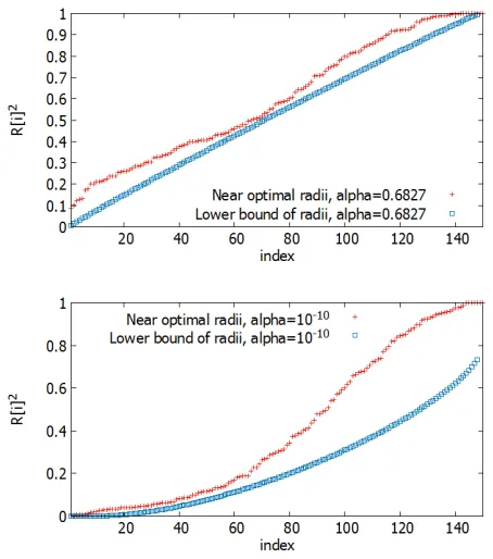
We see that the radii bounds are reasonably tight in both cases. We deduce that in these examples, the enumeration cost bounds will also be tight, because the cost is dominated by what happens aroundk≈n/2.
We note that it is to easier to compute lower bounds than upper bounds.
Fig. 2.Comparison of lower bound and near optimal radii; for the 150-dimensional sim-ulated HKZ basis, compute near optimal radii and lower bound radii forα=0.6827&
P(12,12)(Top) andα=10−10(Bottom).
5.4 Security Estimates for Enumeration
Fig. 1 (in the introduction) displays four bounds on the cost of enumeration in several situations, for varying dimension and simulated HKZ bases and Rankin bases:
– The thin red curve is an upper bound of the enumeration cost usingM = 1010bases with single success probabilityα=10−10computed by the
cross-entropy method.
– The bold red curve is a lower bound of the enumeration cost using M = 1010bases with single success probabilityα=10−10computed byMtimes
– The thin green curve is an upper bound of the enumeration cost w.r.t. in-finitely many bases with global success probabilityα0 =1. This is computed
byM times an upper bound of the enumeration cost with single success probability 1/Mfor a very large M where the single cost is greater than lattice dimension.
– The bold green curve is a lower bound of the enumeration cost w.r.t. in-finitely many bases with a large global success probability. This is computed by (17) withα0 =1.
In all experiments, we take the radius byRn=GH(L). The cost is the number of
nodes of of the enumeration tree in the classical computing model. The security level is the base-2 logarithm of the cost, which is divided by two in the quantum computing model [6,24].
We also draw the curve of 20.292n and 20.265n which are simplified lower
bounds of the cost for solving SVP-nused in [2] for classical and quantum com-puters, respectively.
In all the situations where we use 1010 bases, the upper bounds (thin red curve) and the lower bounds (bold red curve) are close to each other, which demonstrates the tightness of our lower bound.
In the classical setting, our lower bounds for enumeration are higher than sieve lower bounds. On the other hand, in the quantum setting, there are cases where enumeration is faster than quantum sieving. For instance, if an attacker could find many quasi-Rankin bases by some new lattice reduction algorithm, the claimed 2128 quantum security might be dropped to about 296 security. In such a situation, the required blocksize would increase from about 480 to 580.
5.5 Experimental Environments
All experiments were performed by a standard server with two Intel Xeon E5-2660 CPUs and 256-GB RAM. We used the boost library version 1.56.0, which has efficient subroutines to compute (incomplete) beta, (incomplete) gamma and zeta functions with high precision.
Acknowledgements
This work was supported by JSPS KAKENHI Grant Numbers 16H02780, 16H02830 and 18H03238, and JST CREST JPMJCR168A.
References
1. M. Ajtai, R. Kumar, and D. Sivakumar. A sieve algorithm for the shortest lattice vector problem. InProc. of 33rd STOC, pages 601–610. ACM, 2001.
2. M. R. Albrecht, B. R. Curtis, A. Deo, A. Davidson, R. Player, E. Postleth-waite, F. Virdia, and T. Wunderer. Estimate all the {LWE, NTRU} schemes! Posted on the pqc-forum on Feb. 1, 2018. Available at
3. E. Alkim, L. Ducas, T. P ¨oppelmann, and P. Schwabe. Post-quantum key exchange - A new hope. InProc. 25th USENIX Security Symposium, pages 327–343. USENIX Association, 2016.
4. Y. Aono. A faster method for computing Gama-Nguyen-Regev’s extreme pruning coefficients.CoRR, abs/1406.0342, 2014.
5. Y. Aono and P. Q. Nguyen. Random sampling revisited: Lattice enumera-tion with discrete pruning. In Advances in cryptology—EUROCRYPT 2017 Part II, volume 10211 of LNCS, pages 65–102. Springer, 2017. Full version on
https://eprint.iacr.org/2017/155.
6. Y. Aono, P. Q. Nguyen, and Y. Shen. Quantum lattice enumeration and tweaking discrete pruning. https://eprint.iacr.org/2018/546, 2018.
7. Y. Aono, Y. Wang, T. Hayashi, and T. Takagi. Improved progressive BKZ algorithms and their precise cost estimation by sharp simulator.IACR Cryptology ePrint Archive, 2016:146, 2016. Full version of EUROCRYPT 2016.
8. A. Becker, L. Ducas, N. Gama, and T. Laarhoven. New directions in nearest neighbor searching with applications to lattice sieving. InProc. 27th ACM-SIAM Symposium on Discrete Algorithms (SODA), pages 10–24, 2016.
9. D. Cad´e, X. Pujol, and D. Stehl´e. FPLLL library, version 3.0. Available fromhttp: //perso.ens-lyon.fr/damien.stehle, Sep 2008.
10. Y. Chen. R´eduction de r´eseau et s´ecurit´e concr`ete du chiffrement compl`etement homomor-phe. PhD thesis, Univ. Paris 7, 2013.
11. Y. Chen and P. Q. Nguyen. BKZ 2.0: better lattice security estimates. InProc. ASI-ACRYPT 2011, volume 7073 ofLNCS, pages 1–20. Springer, 2011.
12. M.-S. Cheon. Global Optimization of Monotonic Programs: Applications in Polynomial and Stochastic Programming. PhD thesis, Georgia Institute of Technology, 2005. 13. D. Dadush and D. Micciancio. Algorithms for the densest sub-lattice problem. In
Proc. 24th ACM-SIAM Symposium on Discrete Algorithms, SODA 2013, pages 1103– 1122, 2013.
14. P.-T. de Boer, D. P. Kroese, S. Mannor, and R. Y. Rubinstein. A tutorial on the cross-entropy method. Annals of Operations Research, 134(1):19–67, 2005.
15. U. Fincke and M. Pohst. Improved methods for calculating vectors of short length in a lattice, including a complexity analysis. Mathematics of Computation, 44(170):463– 471, 1985.
16. N. Gama, P. Q. Nguyen, and O. Regev. Lattice enumeration using extreme pruning. InAdvances in cryptology—EUROCRYPT 2010, volume 6110 ofLNCS, pages 257–278. Springer, 2010.
17. A. H ¨ulsing, J. Rijneveld, J. M. Schanck, and P. Schwabe. NTRU-HRSS-KEM: Algo-rithm specifications and supporting documentation. NIST submission of Nov. 30, 2017.
18. R. Kannan. Improved algorithms for integer programming and related lattice prob-lems. InProc. 15th ACM STOC, pages 193–206, 1983.
19. D. P. Kroese, S. Porotsky, and R. Y. Rubinstein. The cross-entropy method for contin-uous multi-extremal optimization.Methodology and Computing in Applied Probability, V8(3):383–407, 2006.
20. T. Laarhoven. Sieving for shortest vectors in lattices using angular locality-sensitive hashing. InAdvances in Cryptology - Proc. CRYPTO 2015 - Part I, volume 9215 of
LNCS, pages 3–22. Springer, 2015.
22. D. Micciancio and P. Voulgaris. Faster exponential time algorithms for the shortest vector problem. InProc. ACM-SIAM SODA, pages 1468–1480, 2010.
23. D. Micciancio and M. Walter. Fast lattice point enumeration with minimal overhead. InProc. SODA ’15, pages 276–294, 2015.
24. A. Montanaro. Quantum walk speedup of backtracking algorithms.ArXiv e-prints, 2015.
25. P. Q. Nguyen. Public-key cryptanalysis. In I. Luengo, editor,Recent Trends in Cryp-tography, volume 477 ofContemporary Mathematics. AMS–RSME, 2009.
26. P. Q. Nguyen. Hermite’s constant and lattice algorithms. In The LLL Algorithm: Survey and Applications. Springer, 2010. In [27].
27. P. Q. Nguyen and B. Vall´ee, editors. The LLL Algorithm: Survey and Applications. Information Security and Cryptography. Springer, 2009.
28. P. Q. Nguyen and T. Vidick. Sieve algorithms for the shortest vector problem are practical. J. of Mathematical Cryptology, 2008.
29. M. Pohst. On the computation of lattice vectors of minimal length, successive min-ima and reduced bases with applications.SIGSAM Bull., 15(1):37–44, 1981.
30. R. Y. Rubinstein. Optimization of computer simulation models with rare events.
European Journal of Operations Research, 99:89–112, 1996.
31. R. Y. Rubinstein and D. P. Kroese. The Cross-Entropy Method, A Unified Approach to Combinatorial Optimization, Monte-Carlo Simulation and Machine Learning. Springer-Verlag New York, 2004.
32. M. Schneider and N. Gama. SVP challenge. Available at
http://www.latticechallenge.org/svp-challenge/.
33. C. P. Schnorr. Lattice reduction by random sampling and birthday methods. InProc. STACS 2003, volume 2607 ofLNCS, pages 145–156. Springer, 2003.
34. C.-P. Schnorr and M. Euchner. Lattice basis reduction: improved practical algo-rithms and solving subset sum problems.Math. Programming, 66:181–199, 1994. 35. C.-P. Schnorr and H. H. H ¨orner. Attacking the Chor-Rivest cryptosystem by
im-proved lattice reduction. InProc. of Eurocrypt ’95, volume 921 ofLNCS, pages 1–12. IACR, Springer-Verlag, 1995.
36. U. Shapira and B. Weiss. A volume estimate for the set of stable lattices. Comptes Rendus Math´ematique, 352(11):875 – 879, 2014.
37. J. L. Thunder. Higher-dimensional analogs of Hermite’s constant.Michigan Math. J., 45(2), 1998.
38. S. S. Venkatesh. The Theory of Probability: Explorations and Applications. Cambridge University Press, 2012.
A
Proof of Lemma 3
Let
p(k,n):=Ik/n
k 2,
n−k 2
=
Rk/n
0 z
k
2−1(1−z)n−k2 −1dz
B(2k,n−2k) (18) To prove Lemma 3, it suffices to show that: for any integers 1≤k<n,
p(n,k)≤P(1 2,
1 2) =
R1/2
0 t−1/2e−t
A.1 Formulas and Lemmas
We have
Γ(a+1) =aΓ(a) and B(a,b+1) =B(a,b) b
a+b. (19) The following recurrence formulas hold (see8.17.18and8.17.21ofNIST Digital Library of Mathematical Functionshttp://dlmf.nist.gov/8.17 respec-tively):
Ix(a,b) =Ix(a+1,b−1) +x
a(1−x)b−1
aB(a,b) . (20)
Ix(a,b) =Ix(a,b+1)−x
a(1−x)b
bB(a,b) . (21)
We recall:
Theorem 8. (Chebyshev integral inequality) For any nonnegative, monotonically in-creasing function f(x)and monotonically decreasing function g(x), we have
Z b
a f(x)g(x)dx≤
1 b−a
Z b
a f(x)dx
· Z b a g(x)dx .
Lemma 10. For a,b > 1, the function za(1−z)b is maximized at z
max = a+ab. Furthermore, it is strictly increasing over z ∈ [0,zmax] and strictly decreasing over z∈[zmax, 1].
A.2 Proof Body
The proof of Lemma 3 can be derived from the following three lemmas.
Lemma 11. If n≥2, then: p(1,n)< p(1,n+2).
Proof. By (21), we have
p(1,n) =I1
n
1 2,
n+1 2
−n
−1/2(1−1/n)n−21
n−1 2 ·B
1 2,n
−1 2
= I 1
n+2
1 2,
n+1 2
+
Rn1
1
n+2
z−1/2(1−z)n−21dz B12,n+12
−n
−1/2(1−1/n)n−21
n−1 2 ·B
1 2,n−21
.
ThenJ = p(1,n)−p(1,n+2)is equal to the last two terms. We will show thatJ<0. From (19), we haveB12,n+12 = n−n1B12,n−21and we get
J0= J·(n−1)B
1 2,
n−1 2
=n
Z n1
1
n+2
of which we want to show negativeness.
Since the integral functionz−1/2(1−z)n−21 is strictly decreasing, the trivial
bound
n
Z 1n
1
n+2
z−1/2(1−z)n−21dz
<n 1
n − 1 n+2
1 n+2
−1/2 1− 1
n+2 n−21
= √ 2
n+2
1− 1 n+2
n−21
holds. Thus, letting f(x) = √1
x(1−1/x)
n−1
2 , we have J0 < 2(f(n+2)− f(n))
and it suffices to show that f(x)is strictly decreasing over the rangex∈(n,n+ 2). It is equivalent to check that the derivative of g(x) = f(1/x) = √x(1− x)n−21 is>0 for 1
n+2 <x< 1n. We have: (logg(x))0= g
0(x)
g(x) = 1 2x +
n−1 2
1 x−1 =
nx−1 2x(x−1)
which is>0 if 0<x< 1n. Hence,g(1/(n+2))<g(1/n),f(n+2)< f(n), and
J0= J·(n−1)B
1 2,
n−1 2
=2(f(n+2)−f(n))<0.
Therefore,p(1,n) =p(1,n+2) +J<p(1,n+2)for anyn≥2. ut
Corollary 5. If n≥2, then p(1,n)<P(12,12). Proof. With p(1, 2) = 12 and p(1, 3) = √1
3 ≈ 0.5773 and the known result p(1,n)→P(12,12) (n→∞), we obtain thatp(1,n)<P(12,12)forn≥2. ut
Lemma 12. p(2,n)<P(12,12)for any n≥2 Proof. By definition,
p(2,n) = Γ n
2 Γ(1)Γ n2−1
Z 2n
0
(1−z)n−24dz= n−2
2 Z 2n
0
(1−z)n−24dz
=1−
1− 2
n n2−1
.
For 2≤n≤8, we can check it is smaller than 0.68 numerically, Also, forn≥9, since the function(1−1/x)xis monotonically increasing withx, we have
1−
1− 2 n
n2−1 <1−
1− 2
n n2
Lemma 13. p(k+2,n)< p(k,n)for any1≤k<n.
Proof. By definition and (20)
p(k+2,n)
= Ik+2
n
k 2+1,
n−k 2 −1
=Ik+2
n
k 2,
n−k 2
−2
k
(k+2n )k2(n−k−2
n )
n−k−2 2
B(k2,n−2k)
= p(k,n) +
R k+n2 k n
zk2−1(1−z)n−k2 −1dz
B(k2,n−2k) − 2 k
(k+2n )k2(n−k−2
n )
n−k−2 2
B(2k,n−2k) . Thus, it suffices to show
Z k+n2 k n
zk2−1(1−z)
n−k
2 −1dz−2
k
k+2 n
k2
n−k−2 n
n−k−2 2
:=I−J<0.
Let us define g(z) = zk2+1(1−z)n−k2 −1 which is strictly increasing over
[0,k+2n ]. Sincez−2is strictly decreasing, Chebyshev’s integral inequality implies that
I=
Z k+n2 k n
z−2g(z)dz< n 2
Z k+n2 k n
z−2dz
Z k+n2 k n
g(z)dz= n 2 k(k+2)
Z k+n2 k n
g(z)dz
< n 2 k(k+2)·
2 ng
k+2 n
=J.
Therefore, we haveI< Jand it derivesp(k+2,n)<p(k,n). ut
A.3 Proof of Lemma 9
Recall thatP(a,z):=
Rz
0 xa−1e−xdx
Γ(a) which implies:
e−zza
Γ(a+1) <P(a,z)< za
Γ(a+1) fora>0,z>0. (22)
Also, they imply the bound
P−1(a,x)>(Γ(a+1)x)1/afora>0, 0<x<1 (23) and the limits
lim
z→0+ P(a,z)
za =
1
Γ(a+1) and limx→0+ x
(P−1(a,x))a =
1
Γ(a+1). (24)
Hence, we have
lim
m→∞mVk(
p
βk) =Vk(1)mlim→∞m·
2σ2P−1(k/2,β)
To show the decreasing property, it suffices to show that g(y) = 1y·(P−1(k/2,β0y))k/2is strictly increasing over 0<y≤1.
We use the inequality
∂
∂xP
−1(a,x) =Γ(a)eP−1(a,x)P−1(a,x)1−a ≥ P−1(a,x) ax
which is immediate from the left hand side of (22) withz=P−1(a,x). Hence, denotingP:=P−1(k/2,β0y)for simplicity,
g0(y) = β
0k
2yP
k/2−1·∂P
∂y −
Pk/2 y2 >
β0k
2yP
k/2−1· P (k/2)β0yP
k/2−1− Pk/2 y2 =0