Algorithms for Bohemian Matrices

(1)

Western University Western University

Scholarship@Western

Electronic Thesis and Dissertation Repository

4-5-2019 9:30 AM

Algorithms for Bohemian Matrices

Steven E. Thornton

The University of Western Ontario

Supervisor

Corless, Robert M.

The University of Western Ontario Co-Supervisor Moreno Maza, Marc

The University of Western Ontario

Graduate Program in Applied Mathematics

A thesis submitted in partial fulfillment of the requirements for the degree in Doctor of Philosophy

Follow this and additional works at: https://ir.lib.uwo.ca/etd

Part of the Other Applied Mathematics Commons

Recommended Citation Recommended Citation

Thornton, Steven E., "Algorithms for Bohemian Matrices" (2019). Electronic Thesis and Dissertation Repository. 6069.

https://ir.lib.uwo.ca/etd/6069

This Dissertation/Thesis is brought to you for free and open access by Scholarship@Western. It has been accepted for inclusion in Electronic Thesis and Dissertation Repository by an authorized administrator of

(2)

Abstract

This thesis develops several algorithms for working with matrices whose entries are

multivariate polynomials in a set of parameters. Such parametric linear systems often appear in biology and engineering applications where the parameters represent physical

properties of the system. Some computations on parametric matrices, such as the rank

and Jordan canonical form, are discontinuous in the parameter values. Understanding

where these discontinuities occur provides a greater understanding of the underlying

system.

Algorithms for computing a complete case discussion of the rank, Zigzag form, and the Jordan canonical form of parametric matrices are presented. These algorithms use

the theory of regular chains to provide a unified framework allowing for algebraic or

semi-algebraic constraints on the parameters. Corresponding implementations for each

algorithm in the Maple computer algebra system are provided.

In some applications, all entries may be parameters whose values are limited to finite

sets of integers. Such matrices appear in applications such as graph theory where matrix

entries are limited to the sets{0,+1}, or{−1,0,+1}. These types of parametric matrices can be explored using different techniques and exhibit many interesting properties.

A family of Bohemian matrices is a set of low to moderate dimension matrices where the entries are independently sampled from a finite set of integers of bounded

height. Properties of Bohemian matrices are studied including the distributions of their

eigenvalues, symmetries, and integer sequences arising from properties of the families.

These sequences provide connections to other areas of mathematics and have been archived

in the Characteristic Polynomial Database. A study of two families of structured matrices:

upper Hessenberg and upper Hessenberg Toeplitz, and properties of their characteristic

polynomials are presented.

Keywords: Parametric matrices, Jordan canonical form, Frobenius form, rational

form, Zigzag form, matrix rank, regular chains, parametric linear systems, Bohemian

matrices, random matrices, eigenvalues, upper Hessenberg, Toeplitz, rhapsodic matrices,

Characteristic Polynomial Database.

(3)

Co-Authorship Statement

This integrated-article thesis is based on 5 papers. Chapter 2 has been submitted for

publication, and Chapters 3, and 4 are based on the papers [1], and [2]. For these chapters,

Marc Moreno Maza provided assistance with the theoretical understanding behind regular

chains, and Rob Corless provided assistance with finding applications of the work. A

version of Chapter 5 is being prepared for publication. Rob Corless provided feedback

on the paper. A version of Chapter 6 has been submitted for publication. The initial

basis for this chapter was developed by Rob Corless, Laurenao Gonzalez-Vega, Rafael

Sendra, and Juana Sendra. Eunice Chan provided assistance with compiling the prior

work related to the paper and she generalized work on similar matrices in Theorem 6.5.10.

The work in Sections 6.10 and 6.11 was completed by Rob Corless.

Bibliography

[1] R. M. Corless, M. Moreno Maza, and S. E. Thornton. Zigzag form over families of

parametric matrices. ACM Communications in Computer Algebra, 48(3/4):109–112, Feb 2015.

[2] R. M. Corless, M. Moreno Maza, and S. E. Thornton. Jordan canonical form with

parameters from Frobenius form with parameters. In Proceeding of The International Conference on Mathematical Aspects of Computer and Information Sciences 2017,

pages 179–194. Springer, 2017.

(4)

Acknowledgements

I am grateful for the support of many people who without, this thesis may have never

reached completion.

First, without my Ph.D. supervisors, Rob Corless and Marc Moreno Maza, this thesis

would not have been possible. I thank Rob for giving me the opportunity to pursue

graduate school under his supervision. The knowledge Rob has shared with me over the

past 6 years has been invaluable. I thank Marc for his generosity in sharing his expertise

of regular chains and aiding in the development of several key components of thesis.

Next, I thank my parents, Linda and Scott Thornton, for their constant support

throughout graduate school. Their enthusiasm has kept me going through the course of

my thesis. I am thankful for my partner, Emily Cozens, for helping me stay grounded

throughout graduate school.

I would like to thank my current employer, Rafael Nicolas Fermin Cota, for his

flexibility in allowing me to complete my Ph.D. while concurrently working full time.

After several years of dedication to expanding my knowledge of mathematics, I am

happy to be contributing this thesis to the mathematics community.

(5)

List of Figures

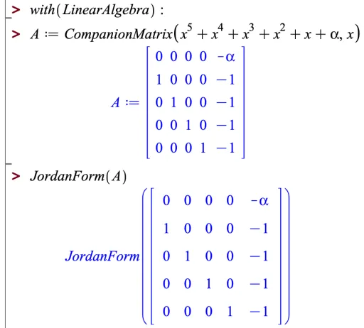
1.1 The JordanForm function in the LinearAlgebra library in Maple fails to compute the Jordan form of a matrix with a single parameter. This

example was run in Maple 2018. . . 2

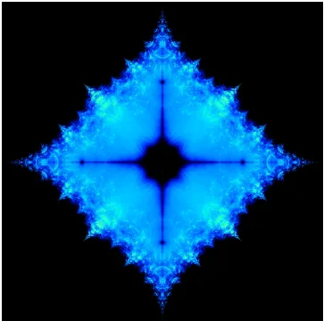
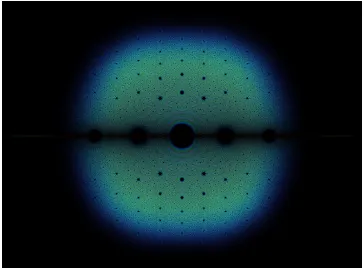
1.2 Density of the eigenvalues of a sample of 100 million tridiagonal matrices

with entries sampled from the set {−1,+1} with entries on the main diagonal fixed at 0. The figure is viewed over the complex range −2−2i

to 2 + 2i. . . 4

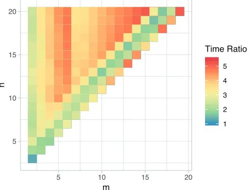
2.1 If A is an m ×n matrix, the color represents the ratio of the time to compute the rank of A over the time to compute the rank of AT_{. The} ratio plotted is an average of the ratios for 100 randomly generatedm×n

matrices with integer entries between −10 and 10, and between 1 and 5

entries containing parameters with at most 5 unique parameters. For each

matrix sampled, the minimum time from 10 iterations is taken. . . 15

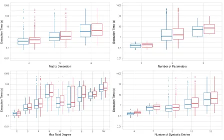
2.2 Bar chart of the execution times for computing the rank of 495 matrices

for our algorithm compared to a naive version. . . 17

2.3 A triangular decomposition into semi-algebraic systems computed with the

RealTriangularizecommand. . . 22 2.4 Output of theRealTriangularize command for the EVE surface. . . 23 2.5 The computed rank values and the corresponding conditions on the

param-eters for Example 1 . . . 24

2.6 The computed rank values and the corresponding conditions on the

param-eters for Example 2 (part 1) . . . 25

param-eters for Example 2 (part 2) . . . 26

param-eters for Example 3 . . . 26

4.1 Our implementation provides a full case discussion of the JCF of a matrix

with 5 parameters. Two non-trivial cases are shown. . . 34

(10)

4.2 Time to compute the JCF of each Frobenius form in the full case discussion

of the Frobenius form of the matrix in section 4.6.2. For alln, the Frobenius form splits into two cases: ρ = 0 and ρ6= 0. The JCF is computed over each of these branches. Note the exponential growth. Timing was done

on a 2016, 3.3GHz quad-core Intel Core i7 iMac with 16GB of RAM using

Maple 2016.2. . . 45

5.1 Density plot over the complex plane of the eigenvalues of all 5×5 matrices

with entries from the set {−1,0,+1}. The plot is viewed on −4.13−3.1i

to 4.13 + 3.1i. . . 53 5.2 The roots of all degree 25 polynomials with±1 coefficients. . . 54

5.3 Examples of structures appearing in the plots of Bohemian eigenvalues. . 62

5.4 Radius of the spectrum for the Bohemian family ofn×n upper Hessenberg matrices with a Toeplitz structure, entries on the main diagonal fixed at 0,

and population {−1,+1}. Radius values for dimensions 3 to 25 are exact. For dimensions larger than 25 the radius has been approximated from a

sample of 100 million matrices at each dimension. All computations were

performed in double precision. . . 63

5.5 Density plot in the complex plane of the eigenvalues of a random sample

of matrices from the Bohemian family of 5×5 matrices with population {−1,0,+1}. . . 65 5.6 Eigenvalues from the family of 5×5 Bohemian matrices with population

{−1,0,+1}. The left half contains the eigenvalues from a sample of 100 million matrices and the right half contains the eigenvalues from

all 325_{= 847}_,₂₈₈_,₆₀₉_,_{443 matrices in the family. . . .} ₆₆ 5.7 A histogram of the densities in the bins (pixels) for the family of 5×

5 matrices with population {−1,0,+1} over the 2001×2001 pixel grid ranging from−4−4i to 4 + 4i. The bin with the highest density contains 296,330,735,533 eigenvalues and is the bin that contains 0. The lowest

density bins only contain 160 eigenvalues and occurs 4 times in the density

matrix. Bins containing 3,840 eigenvalues are the most common (excluding

bins with no eigenvalues) and occur 78,440 times in the density matrix. . 72

5.8 Time to compute and plot the eigenvalues of 1 million matrices for a range

of matrix dimensions. Computations were done using 16 cores on an AMD

Ryzen Threadripper 1950X 16 core/32 thread 3.7GHz with 64GB of RAM. 73

(11)

5.9 Numeric error in multiple eigenvalues at 0 for two families of matrices.

Red circles have been added to show the expected error in an eigenvalue of

multiplicity m at 0 of ε1/m where ε is machine epsilon. . . 77

6.1 The set of eigenvalues of all 10,460,353,203 six by six upper Hessenberg matrices H with entries Hi,j ∈ {−1,0,+1} for 1 ≤ i ≤ j ≤ 6, and

Hi+1,i = 1 for 1 ≤ i < 6. A more detailed image can be found at

assets.bohemianmatrices.com/gallery/UH_6x6.png . . . 92 6.2 The set of eigenvalues of all 14×14 upper Hessenberg Toeplitz matrices with

sub-diagonal entries equal to 1, and all other entries from the set{−1,0,+1}. A more detailed image can be found at assets.bohemianmatrices.com/ gallery/UHT_14x14.png . . . 92 6.3 The set of eigenvalues of all 14,348,907 matrices inZ6×6

{0} ({−1,0,+1}); that is, six by six upper Hessenberg matrices Hwith entries Hi,j ∈ {−1,0,+1} for 1≤ i < j ≤ 6, diagonal entries fixed as zero, and Hi+1,i = 1 for 1≤

i <6. A more detailed image can be found at assets.bohemianmatrices. com/gallery/UH_0_Diag_6x6.png . . . 93 6.4 The set of eigenvalues of all 14×14 upper Hessenberg Toeplitz matrices

sub-diagonal entries equal to 1, diagonal entries equal to 0, and all other

entries from the set{−1,0,+1}. A more detailed image can be found at

assets.bohemianmatrices.com/gallery/UHT_0_Diag_14x14.png . . . 93 6.5 The points are logτn+1 −logτn for n from 0 to 50,000 where τn is the

maximal characteristic height ofMn×n _{(i.e. when} _t

k =−1, for example). The solid line is log(1 +ϕ) where ϕis the golden ratio. . . 110 6.6 Degree of the term corresponding to the height of the characteristic

polyno-mial of ann×nupper Hessenberg Toeplitz matrix of maximal characteristic height. . . 111

(12)

List of Tables

5.1 For the Bohemian family of n×n matrices with population {−1,0,+1}, the table reports the number of matrices (3n2

), the number of distinct

characteristic polynomials, and the number of distinct eigenvalues. . . 56

5.2 For the Bohemian family of n×n matrices with population {−1,0,+1}, the table reports the number of matrices (3n2

), the number of strictly

rhapsodic matrices, and the number of non-strictly rhapsodic matrices. . 57

5.3 Permutation symmetries for the Bohemian familyMofn×nmatrices with population {−1,0,+1}. The #Mcolumn gives the number of matrices in the family, #MP gives the number of matrices in a permutation normal subset ofM, and #MO gives the number of matrices in the subset of M

with entries ordered along the diagonal. The log₁₀ 1− #M n!#MP

column

shows the convergence of the permutation normal subset to the bound

given in Proposition 5.3.17. . . 59

5.4 Number of distinct characteristic polynomials and Jordan canonical forms

(JCFs) for the family of n×n matrices with population{−1,0,+1}. The number of distinct Jordan forms for the 5×5 family is currently unknown. 61

(13)

5.5 Comparison of the time (in seconds) to sample and compute the eigenvalues

of 1 million 5×5 matrices with population {−1,0,+1}inMatlab, Python (NumPy), and Julia. The “Sample and Eigenvalues” column gives the time

taken to sample and compute eigenvalues, the “Sample” column is the time

to sample 1 million matrices, and the “Eigenvalues” column gives the time

to compute the eigenvalues of a matrix 1 million times. The “Eigenvalues”

column is based on computing the eigenvalues of a matrix 1 million times

and is repeated for a sample of 100 matrices. The average time is given.

The “Python (NumPy) Sequential” row gives the time to repeatedly sample

5×5 matrices and then compute their eigenvalues whereas the “Python

(NumPy) Batched” row gives the time to sample a single array of dimension

1,000,000×5×5 and use the batched functionality of thenumpy.linalg.eig

function to compute the eigenvalues of all matrices with only one function

call. All scripts were run on a single thread on a computer with an AMD

Ryzen Threadripper 1950X 16 core/32 thread 3.7GHz processor and 64GB

of RAM using Matlab R2018a, Python 3.6.2 (NumPy 1.13.1), and Julia

1.0.2. . . 74

6.1 Some properties of matrices inHn×n

{0} ({−1,0,+1}). The #matrices column reports the number of distinct matrices at each dimension. The #cpolys

column reports the number of distinct characteristic polynomials at each

dimension. The #neutral polys reports the number of characteristic

poly-nomials where all roots have zero real part. The #neutral matrices column

reports the number of matrices where all eigenvalues have zero real part. 96

6.2 Some properties of matrices in Z_{n₀×_}n({−1,0,+1}). The #matrices column reports the number of distinct matrices at each dimension. The #cpolys

dimension. The #neutral polys reports the number of characteristic

poly-nomials where all roots have zero real part. The #neutral matrices column

reports the number of matrices where all eigenvalues have zero real part. 97

6.3 Number of distinct eigenvalues of various multiplicities of matrices in Zn×n

{0} ({−1,0,+1}). Most eigenvalues are simple. It turns out that every multiple eigenvalue also occurs as a simple eigenvalue for some other matrix.

The only n-multiple eigenvalue of the class ofn by n matrices is, of course,

λ= 0. . . 97

(14)

6.4 Some properties of matrices in Hn×n

{0} ({0,+1}). The #matrices column reports the number of distinct matrices at each dimension. The #cpolys

dimension. The #distinct real λ column reports the number of distinct real eigenvalues inHn×n

{0} ({0,+1}). The #neutral polys reports the number of characteristic polynomials where all roots have zero real part (here only

zn_{). We conjecture that this is always so (and that there is only one matrix} for that neutral polynomial). The #neutral matrices column reports the

number of matrices where all eigenvalues have zero real part. . . 98

6.5 Number of distinct eigenvalues of various multiplicities matrices inHn×n

{0} ({0,+1}). Note that in this class of matrices, diagonal entries of the matrix need not

be zero. . . 98

6.6 Some properties of matrices from Hn_{₀×_}n({−1,+1}). The column #stables reports the number of characteristic polynomials with all roots in the left

half plane; the corresponding number ofmatrices is 1, 4, 28, 424, and 11,613. Other columns are as in previous tables. Blank table entries represent

unknowns. . . 99

6.7 Number of distinct eigenvalues of various multiplicities of matrices from Hn×n

{0} ({−1,+1}). The diagonal entries are not zero. . . 99 6.8 Maximum height, τn, degree of term of characteristic polynomial

corre-sponding to maximum height, µn, and the number of matrices in Mn×n for dimensions 2 to 10. . . 109

6.9 The numbers of Type I stable matrices for various populations and

dimen-sions. . . 129

6.10 The numbers of nilpotent matrices for various populations and dimensions 130

(15)

Abbreviations

CAS Computer algebra system

CPDB Characteristic polynomial database

GCD Greatest common divisor

JCF Jordan canonical form

OEIS Online Encyclopedia of Integer Sequences

(16)

Chapter 1 Introduction

1.1 Parametric Linear Systems

Linear systems are a universal tool in mathematics with their use spanning nearly all

applications. Many applications contain parameters that may be unknown quantities, or

approximate values found through experimentation. The values the parameters take may

lead to a significant difference in the meaning of the underlying system. Understanding

the influence of the parameter values on the underlying system is of great interest. Solving

linear systems with parameters has been studied extensively with early work by Sit in [2].

Significantly less work has been done on computing other properties of these systems

such as the distribution of rank as a function of the parameters, or the possible Jordan

canonical forms (JCF).

Many computer algebra systems (CAS) struggle with these types of problems. Asking

for the rank of a parametric matrix in Maple for example will return a generic solution

assuming the parameter values are transcendental numbers. For example, for the matrix

A= 

 

1 2 3

4 5 6

7 8 α



 

where α ∈ _C, Maple will compute the rank to be 3. If we specialize α = 9, we find that the rank is 2. Even worse, in Maple, asking for the JCF of a parametric matrix

whose characteristic polynomial cannot be factored such that all irreducible terms are of

degree less than 5 will simply fail to provide a solution, see Figure 1.1 for example. These

problems appear to be universal across CAS. Sometimes the implementations will warn

the user that the answer may not be correct for all parameter values. In the Sage CAS

(17)

Chapter 1. Introduction 2

for example, a user is warned when computing the JCF of a parametric matrix and the

generic solution is provided. Solving parametric linear systems have been more successful

in those CAS with many specialized packages developed for working with these systems.

Figure 1.1: The JordanForm function in the LinearAlgebra library in Maple fails to compute the Jordan form of a matrix with a single parameter. This example was run in Maple 2018.

In this thesis, methods for analyzing matrices with entries that are multivariate

polynomials in a set of parameters are developed. Initially motivated by the failures

of _Maple when computing the JCF of a parametric matrix, several algorithms are

developed including one for the JCF where the input matrix is in Frobenius form and

contains polynomial entries. The complexity of these problems is high when parameters

are present. As such, the algorithms are typically limited to small systems with few

parameters. They may succeed on larger systems but this success is dependent on the

linear system. A Maple package called ParametricMatrixToolshas been developed to share the algorithms with the greater mathematics community. These algorithms have

been developed using the theory of regular chains [1] and the ParametricMatrixTools

package has been built on top of the RegularChains package.

Some applications contain matrices where all entries are parameters. Further, such

parameter values may be restricted to belonging to small sets of integers. Such matrices

appear in graph theory where the entries are restricted to the sets {0,+1}, or{−1,0,+1}. Since the entries are restricted to small sets, different approaches may be used for the

(18)

matrices that all matrices can be exhaustively explored. Relationships within these

families can further reduce the computation required for many properties. Exploring these

families of parametric matrices turns out to be a very interesting problem on its own.

1.2 Bohemian Matrices

Low dimension square integer matrices are commonly used in introductory linear algebra

curricula for teaching the fundamental concepts. These matrices are often used as examples

for analyzing linear systems including solving the system, and computing its eigenvalues.

Despite their simplicity, many questions remain about these low dimension matrices. For

example, how many singular 6×6 matrices with entries from the set {−1,0,+1}exist? To date the answer is unknown. While the computation for a single matrix is simple,

and is not outside of the scope of what an undergraduate student should be able to

compute, the difficulty comes from the number of such matrices. For this example there

are 336 _{= 150}_,₀₉₄_,₆₃₅_,₂₉₆_,₉₉₉_,_{121 matrices, most of which have likely never appeared} on a linear algebra exam. Even with modern computing power, questions like these still

remain outside the scope of what can be computed on standard hardware. Since the

number of matrices grows exponentially in the square of the dimension, computational

hardware will never be able to make much progress on these problems.

The study of Bohemian matricesfocuses on answering questions about distributions

of low dimension integer matrices with entries of bounded height. A Bohemian family

is a distribution of Bohemian matrices where the population is the set of integers the

entries are sampled from. Inspiration for studying these types of problems originated

when exploring density plots of the eigenvalues of such types of random matrices. Discrete

structures appear in the eigenvalue densities that do not have obvious explanations, see

Figure 1.2 for example.

The exploration of new Bohemian families typically begins with plotting the density of

the eigenvalues in the complex plane. To ease this exploration phase, aMatlabframework

was developed to assist with generating mathematically accurate plots. This framework

has been made available at https://github.com/BohemianMatrices/BHIME-Project. Specializing to Bohemian families where the matrices are structured (e.g. upper

Hessenberg, Toeplitz, circulant, etc.) has shown to be more successful in developing

an understanding of relationships within these families. With these special structures,

existing work on such structured matrices can be extended by restricting the entries to

belong to a small population of integers. Further, brute force exploration can help identify

(19)

Figure 1.2: Density of the eigenvalues of a sample of 100 million tridiagonal matrices with entries sampled from the set{−1,+1} with entries on the main diagonal fixed at 0. The figure is viewed over the complex range−2−2i to 2 + 2i.

Brute force computation over Bohemian families can also be used to find the

distribu-tions of characteristic polynomials. In many families, the size of the set of characteristic

polynomials is substantially smaller than the set of matrices. Thus, for some questions,

working with the set of characteristic polynomials can be easier than with the family of

Bohemian matrices. For example, the distribution of determinants within a family can

be read directly from the characteristic polynomials. Questions like this have inspired

the development of the Characteristic Polynomial Database (CPDB). The CPDB

provides distributions of the characteristic polynomials for families of Bohemian

matri-ces. The database is publicly available at http://www.bohemianmatrices.com/cpdb/

and currently contains 1,762,728,065 characteristic polynomials from 2,366,960,967,336

(20)

1.3 Outline

This thesis begins with three chapters on algorithms for parametric matrices. In Chapters 2

through 4, algorithms for computing the rank, Zigzag form, Frobenius (rational) form and

Jordan form of parametric matrices are discussed. Chapters 5 and 6 focus on Bohemian

matrices. Chapter 5 provides a general discussion of Bohemian matrices followed by a

detailed study of a specific family of Bohemian matrices in Chapter 6.

Chapter 2 presents an algorithm for computing the rank of a parametric matrix as a

function of the parameters while avoiding explicitly solving the corresponding parametric

linear system. As input, this algorithm takes a matrix with multivariate polynomial

entries whose indeterminates are regarded as parameters and are subject to a system

of polynomial equations and inequalities. The algorithm relies on the theory of regular

chains. An implementation of the algorithm in the Maplecomputer algebra system is

presented, which has been built on top of the RegularChains library. The effectiveness of the implementation is demonstrated by comparing it to a na¨ıve implementation and by

using it to find the rank of several examples from the literature.

In Chapter 3, an algorithm for computing the Zigzag form of a parametric matrix as a function of the parameters is presented. This work was motivated by a desire to compute

the Frobenius (rational) canonical form of a parametric matrix. By first computing the

Zigzag form, the Frobenius form can be obtained by GCD computations. The algorithm

for the constant case has been taken from [3] and has O(n3_{) complexity. This algorithm} has been modified to provide a full case discussion for matrices with parameters.

Chapter 4 introduces an algorithm for computing the JCF of a parametric matrix

that is in Frobenius form. The algorithm takes as input a matrix in Frobenius canonical

form where the entries are multivariate polynomials in the parameters and computes a

complete case discussion for the JCF. The JCF of a square matrix is a foundational tool

in matrix analysis. If the matrix A is known exactly, symbolic computation of the JCF is

possible though expensive. When the matrix contains parameters, exact computation

requires either a potentially very expensive case discussion, significant expression swell, or

both. For this reason, no current computer algebra system will compute a case discussion

for the JCF of a matrix A(α) where α is a (vector of) parameter(s). This problem is extremely difficult in general, even though the JCF is encountered early in most curricula.

The algorithm presented is based on the theory of regular chains and an implementation

built on the RegularChainslibrary in Maple is discussed.

Chapter 5 addresses some of the interesting features of Bohemian families including

(21)

BIBLIOGRAPHY 6

Matlab framework for visualizing distributions of eigenvalues is presented and used as an experimental tool for understanding discrete structures found in these distributions.

While developing the framework, two families of Bohemian matrices were found where the

Matlabeigenvalue solver fails to produce solutions in some instances. The techniques used for computing the properties and characteristic polynomials found in the Characteristic

Polynomial Database are introduced.

Chapter 6 explores a special family of Bohemian matrices, specifically those with entries

from the set {−1,0,+1}. More, these matrices are specialized to be upper Hessenberg, with sub-diagonal entries ±1. Many properties remain after these specializations, some of

which were surprising. Two recursive formulae for the characteristic polynomials of upper

Hessenberg matrices are given. Focusing on only those matrices whose characteristic

polynomials have maximal height allows us to explicitly identify these polynomials and

give a lower bound on their height. This bound is exponential in the order of the matrix.

We count stable matrices, normal matrices, and neutral matrices, and tabulate the results

of our experiments. We prove a theorem about the only possible kinds of normal matrices

amongst a specific family of Bohemian upper Hessenberg matrices.

Bibliography

[1] P. Aubry, D. Lazard, and M. Moreno Maza. On the theories of triangular sets. Journal of Symbolic Computation, 28(1-2):105–124, 1999.

[2] W. Y. Sit. An algorithm for solving parametric linear systems. Journal of Symbolic Computation, 13(4):353–394, 1992.

[3] A. Storjohann. An O(n3_{) algorithm for the Frobenius normal form. In} _Proceedings

(22)

Chapter 2 Comprehensive Rank Computation

for Matrices Depending on

Parameters

2.1 Introduction

Determining the rank of a matrix is a simple computation traditionally presented in

introductory linear algebra courses. Unfortunately, the computation for parametric

matrices is a tedious process which, to our knowledge, does not yet have a completely

satisfactory solution. In this paper we present an algorithmic approach to extending the

methods of rank computation to parametric matrices with polynomial entries. External

equality and inequality constraints on the parameters may be inherited in the problem

being solved and will be considered in the computations. Additionally, we present an

implementation of our algorithm in the Maple computer algebra system (CAS).

For an m ×n matrix A(α), where the parameters α are subject to a system of polynomial constraints S, our rank computation proceeds as follows. We compute the null space of A(α) by means of a triangular decomposition of the polynomial system S0

obtained by adding to S the equations of A(α)X = 0, where X is a column vector of unknowns x1, . . . , xn. By means of set-theoretic operations on algebraic or semi-algebraic sets, we deduce a decomposition of the parameter space into cells C0, . . . , Cn such that aboveCr, for all 0≤r≤nthe rank ofA(α) is equal tor. The proposed method is, in fact, stated for both algebraic and semi-algebraic constraints. This feature is achieved thanks

to the theory of regular chains which provides us with a unified framework, reviewed in

Section 2.2, for solving polynomial systems over both the complex and the real numbers.

(23)

Chapter 2. Comprehensive Rank of Matrices Depending on Parameters8

In addition, the proposed method is tailored to the problem of parametric matrix

rank computation. That is, we avoid the usage of general tools for solving parametric

polynomial systems, such as comprehensive Gr¨obner bases [22], comprehensive triangular decomposition[8], ordynamic evaluation[4, 12]. In fact, we rely on the non-comprehensive triangular decomposition algorithms presented in [9] and [6] for the complex and real

cases, respectively.

Our approach is presented in Section 2.4, following two lemmas established in

Sec-tion 2.3. We implemented our algorithms in the Maple CAS. Section 4.6 reports on

the successful application of our implementation to various examples taken from the

literature. In addition, the experimental part of our work revealed the importance of a

tailored method, that is, a method avoiding general tools for solving parametric

polyno-mial systems. Indeed, a preliminary implementation, based on comprehensive triangular

decomposition, was generating much more complex output and was substantially slower

than the method presented in Section 2.4.

Works related to this paper include polynomial eigenvalue problems [18, 21] which are

sub-problems of the question studied in this paper. In addition, control theory, where the

rank of a real matrix can be used to determine whether a linear system is controllable, or

observable, is an important area of applications for parametric matrix rank computation.

Extensive work has been done on solving parametric linear systems [2, 11, 13, 17], with

some of the earliest work done by William Sit [20].

2.2 Preliminaries

The algebraic material reviewed below supports the algorithm presented in Section 2.4.

The notion of a regular chain, introduced independently in [16] and [23], is closely related to that of a triangular decomposition of a polynomial system. Broadly speaking, a

triangular decomposition of a polynomial systemS is a set of simpler (in a precise sense) polynomial systems S1, . . . , Se such that a point p is a solution ofS if, and only if,p is a solution of (at least) one of the systems S1, . . . , Se.

When the purpose is to describe all the solutions of S, whether their coordinates are real numbers or not, in which case S is said to be algebraic, those simpler systems are required to be regular chains. We refer to [1, 9] for a formal presentation on the concepts

of a regular chain and a triangular decomposition of an algebraic system.

(24)

in [6]. In both cases, each of these simpler systems has a triangular shape and remarkable

properties, which justifies the terminology.

Multivariate polynomials. Let_K be a field. If _Kis an ordered field, then we assume

that it is a real closed field like the field_R of real numbers. Otherwise, we assume that _K

is algebraically closed, like the field _Cof complex numbers. Let X1 <· · ·< Xs be s≥1 ordered variables. We denote by _K[X1, . . . , Xs] the ring of polynomials in the variables

X1, . . . , Xs with coefficients in K. For a non-constant polynomial p∈K[X1, . . . , Xs], the greatest variable inpis called themain variableofp, denoted by mvar(p), and the leading coefficient of p w.r.t. mvar(p) is called the initial of p, denoted by init(p).

Regular chains. A set R of non-constant polynomials in _K[X1, . . . , Xs] is called a triangular set, if for all p,q ∈R with p6=q we have mvar(p)6= mvar(q).A variable Xi is said to be freew.r.t. R if there exists no p∈R such that mvar(p) =Xi. For a nonempty triangular set R, we define thesaturated idealsat(R) of R to be the idealhRi:h∞_R, where

hR is the product of the initials of the polynomials inR. The saturated ideal of the empty triangular set is defined as the trivial idealh0i. From now on,R denotes a triangular set of K[X1, . . . , Xs]. The ideal sat(R) has several properties, and in particular it is unmixed [3]. We denote its height, that is, the number of polynomials in R, by e, thus sat(R) has dimension s−e. Let Xi1 < · · · < Xie be the main variables of the polynomials in R.

We denote by rj the polynomial of R whose main variable is Xij and by hj the initial

of rj. ThushR is the product h1· · ·he. We say thatR is a regular chain whenever R is empty or, {r1, . . . , re−1} is a regular chain and he is regular modulo the saturated ideal sat({r1, . . . , re−1}).

Constructible sets. LetF ⊂_K[X1, . . . , Xs] be a set of polynomials andg ∈K[X1, . . . , Xs] be a polynomial. We denote by V(F) ⊆_Ks _the _{zero set} _or _{affine variety} _of _F_{, that is,} the set of points in the affine space_Ks _{at which every polynomial} _f _∈_F _{vanishes. If} _F consists of a single polynomial f, we write V(f) instead of V(F). We call a constructible set any subset of _Ks of the form V(F)\V(g). LetR ⊂_K[X1, . . . , Xs] be a regular chain and leth∈_K[X1, . . . , Xs] be a polynomial. We say that the pair [R, h] is aregular system whenever h is regular modulo sat(R) and V(hR) ⊆ V(h) holds. We write Z(R,h) for

V(R)\V(h). One should observe that for a regular system [R, h] the zero set Z(R,h) is necessarily not empty. Regular systems provide an encoding for constructible sets.

More precisely, there exists a finite family T of regular systems [R1, h1], . . . ,[Re, he] of K[X1, . . . , Xs] such that

(25)

We call T atriangular decomposition of the constructible set V(F)\V(g). In the sequel of this section, we assume that _K is a real closed field.

Regular semi-algebraic systems. A regular semi-algebraic system of _K[X1, . . . , Xs] is a triple [T, Q, P] where T ⊂ _K[X1, . . . , Xs] is a regular chain, Q is a quantifier-free formula involving only the free variables of T andP is a set of positive inequalities defined by polynomials of _K[X1, . . . , Xs]; moreover [T, Q, P] must satisfy the following properties:

(i) Q defines a non-empty open set in the space of the free variables of T;

(ii) at any point α defined by Q, the product hT of the initials of T does not vanish, the specialized regular chain Tα generates a radical ideal and, each specialized polynomial in Pα is invertible modulo the ideal generated by Tα;

(iii) at any point α defined by Q, the specialized semi-algebraic system [Tα, Pα] admits at least one real solution β, that is, every polynomial inTα is zero at β, and every polynomial in Pα is positive at β.

We denote by Z(T, Q, P) the set of the points in the affine space _Ks _{simultaneously} satisfying the quantifier-free formula Q, the equation f = 0 for each f ∈T and, each of the inequalities of P.

Semi-algebraic sets. We call a semi-algebraic system of _K[X1, . . . , Xs] any polynomial system S of the form

f1 =· · ·=fa= 0, g 6= 0, p1 >0, . . . , pb >0, q1 ≥0, . . . , qc≥0,

where f1, . . . , fa, g, p1, . . . , pb, q1, . . . , qc are polynomials of K[X1, . . . , Xs]. The solution set S consists of all points in the affine space _Ks satisfying simultaneously the above constraints. We call a semi-algebraic set any subset of _Ks _{which is the solution set of} a semi-algebraic system of _K[X1, . . . , Xs]. Regular semi-algebraic systems provide an encoding for semi-algebraic sets. More precisely, there exists a finite family T of regular

semi-algebraic systems [T1, Q1, P1], . . . , [Te, Qe, Pe] of K[X1, . . . , Xs] such that we have

S = Z(T1, Q1, P1) ∪ · · · ∪ Z(Te, Qe, Pe).

We call T a triangular decompositionof the semi-algebraic set S. Examples are provided in Appendix 2.6. An important property of any regular semi-algebraic system [T, Q, P] is the fact that it is a parametrization of its zero set. Therefore, a triangular decomposition

of a semi-algebraic system S decomposes the zero set ofS into components, each of which is given by a parametric representation. This encoding of a semi-algebraic set is very

(26)

Encoding constructible sets (resp. semi-algebraic sets) with regular systems (resp.

regular semi-algebraic systems) has another benefit. It leads to efficient algorithms for

performing set-theoretic operations on constructible and semi-algebraic sets; see [8] and [7]

respectively. These operations, as well as the above mentioned triangular decomposition

algorithms, are part of theRegularChainslibrary [5, 19] distributed with theMapleCAS. In Section 2.4, our algorithm refers to the operationsTriangularize,RealTriangularize

and Difference of the RegularChains library. The first two operations compute a triangular decomposition of a constructible set and a semi-algebraic set, respectively. The

latter applies to a couple (A,B), of either constructible sets or semi-algebraic sets, and returns the set-theoretic difference A\B.

2.3 Lemmas

We use the same notations as in Section 2.2. In addition, we consider k ≥ 1 ordered variablesα1 <· · ·< αk that we shall view as parameters. LetA(α) =A(α1, . . . , αk) be anm×n matrix with coefficients in_K[α1, . . . , αk].

If _K is a real closed field, we assume that α1, . . . , αk are subject to a semi-algebraic system S defined by polynomials of _K[α1, . . . , αk]. We denote by Σ ⊆ Kk the semi-algebraic set defined by S. If _K is algebraically closed, we assume that α1, . . . , αk are subject to an algebraic system that we denote by S and which is defined by polynomials of _K[α1, . . . , αk]. We denote by Σ ⊆Kk the corresponding constructible set.

Our aim is to compute the rank of A(α) for all α ∈ Σ. More precisely, we aim at decomposing Σ into cells C0, . . . , Cn such that the rank of A(α) is r for all α ∈Cr, for 0≤r≤n.

Let X be ann-element column vector whose entries are ordered variables x1, . . . , xn satisfying α1 < · · · < αk < x1 < · · · < xn. Denote by Π the standard projection from Kk+n onto the space of the least k coordinates. We consider the polynomial system S0 obtained by adding to S the equations of A(α)X = 0. These are equations given by polynomials of _K[α1 <· · ·< αk < x1 <· · ·< xn]. Let T be a triangular decomposition of the zero set of S0. The following two lemmas state respectively in the complex and real cases a key property which allows us to deduce from T a case discussion for the

computation of the null space of A(α). This will be used in Section 2.4 in order to obtain the desired parametric rank computation.

Lemma 2.3.1. If _K is algebraically closed, then T is a finite family of regular systems

(27)

(i) each polynomial in each regular chain T1, . . . , Te has degree zero or one w.r.t. each of the variables x1, . . . , xn;

(ii) each polynomial hi belongs to K[α1, . . . , αk];

(iii) for each1≤i≤e, the projection Π(Z(Ti, hi)) is given byZ(Ti ∩ K[α1, . . . , αk], hi), that is,

Π−1(Π(Z(Ti, hi))) =Z(Ti ∩ K[α1, . . . , αk], hi),

thus, Π(Z(Ti, hi)) is obtained by “erasing” from [Ti, hi] those polynomials where at least one of the variables x1, . . . , xn appears.

Proof. We first prove (i). Since variables are ordered as α1 <· · ·< αk < x1 <· · ·< xn and since the input polynomials have degree zero or one w.r.t. each of the variables

x1, . . . , xn, the triangular decomposition algorithm of [9] (which relies on polynomial GCD and resultant computations) generates polynomials which all have degree zero or one

w.r.t. each of the variables x1, . . . , xn. This observation implies (i). Next, we prove (ii). Following again the triangular decomposition algorithm of [9], each of the polynomials

h1, . . . , he comes either from the input systemS0 or, is a factor of an initial or, a factor of a resultant computed by the triangular decomposition algorithm of [9]. It follows from

(i) that each of h1, . . . , he necessarily belongs to K[α1, . . . , αk]. Finally, we prove (iii). Let [Ri, hi] be any of the regular systems ofT. Let β be a point in the parameter space. Since hi does not involve any of the variables x1, . . . , xn the inequationhi(β)6= 0 makes sense. Since hi(β)6= 0 implies that none of the initials of Ti vanishes at β, the conditions

hi(β)6= 0 and f(β) = 0 (∀f ∈Ti ∩ K[α1, . . . , αk]),

are sufficient for β to be extended to a zero of Z(Ti, hi). The conclusion follows. \

Lemma 2.3.2. If _K is a real closed field, then T is a finite family of regular semi-algebraic systems [T1, Q1, P1], . . . ,[Te, Qe, Pe] of K[α1, . . . , αk, x1, . . . , xn] such that the following properties hold:

(1) each polynomial in each regular chain T1, . . . , Te has degree zero or one w.r.t. each of the variables x1, . . . , xn;

(2) each set of polynomial inequalities Pi is empty; (3) for each i= 1· · ·e, we have

(28)

Proof. A first step is to compute a triangular decomposition T

K over the algebraic closure

of _K of the system S00 consisting only of the equations of S0. (See Line 1 of Algorithm 2 in [6].) Lemma 2.3.1 applies to S00 and T_K. Hence T_K consists of regular systems [T1, h1], . . . ,[Te, he] satisfying properties (i), (ii) and (iii) of Lemma 2.3.1. A second step is to refine T_K (still over the algebraic closure of _K) by using the inequations and

inequalities of S0 as inequations. (See Lines 2 to 15 of Algorithm 2 in [6].) Since S0

has no inequations or inequalities involving (at least one of) the variables x1 <· · ·< xn, we can still assume that, after this second step, we have a triangular decomposition

consisting of regular systems [T1, h1], . . . ,[Te, he] satisfying properties (i), (ii) and (iii) of Lemma 2.3.1. A third and final step is, for each regular system [Ti, hi], to check whether or not it has real solutions and, if yes, to generate the quantifier free Qi such that the regular semi-algebraic system [Ti, Qi,∅] describes those real solutions (See Lines 16 to 19 of Algorithm 2 together with Algorithms 3, 5 and 6 in [6].) One should observe that

each Qi may contain inequalities. However, those inequalities involve the parameters

α1, . . . , αk only. Claims (1) and (2) follow from the above observations. Finally, Claim (3) follows from Claims (1) and (2) and the properties of a regular semi-algebraic system. \

Lemmas 2.3.1 and 2.3.2 imply that the Π-projections of the zero sets of the regular

systems (resp. regular semi-algebraic systems) of the triangular decomposition T

decom-pose the constructible set (resp. semi-algebraic set) Σ into cells B0, . . . , Be above which the solutions of the parametric linear system A(α)X = 0 is given by one of the regular systems inT. However, this does not yet solve our parametric rank computation problem.

Indeed, the solution set ofA(α)X = 0 above a cell Bi might be contained into the solution set of A(α)X = 0 above another cell Bj, for some 0≤i < j ≤e. In fact, dealing with redundant components is a well-known issue in all types of algorithms for decomposing

polynomial systems. This difficulty is handled in Section 2.4 by a post-processing of the

triangular decomposition T.

2.4 Algorithm

Reusing the notations of Section 2.3, recall that T is a triangular decomposition of the

zero set of the systemS0 obtained by adding to S the equations ofA(α)X = 0, whereS

is a polynomial system on the parameters of the m×n parametric matrix A(α). The following procedure computes a decomposition of the zero set Σ ⊆ _Kk _of _S _{into cells}

(29)

in Section 2.2. Assume first that _K is algebraically closed.

Step 1: LetT := Triangularize(S0,_K[α1 <· · ·< αk< x1 <· · ·< xn])

Step 2: For 0≤r≤n, letCr be the constructible set of Kk given by all regular systems [Tj ∩ K[α1 <· · ·< αk], hj] such that [Tj, hj]∈ T and the number of polynomials of Tj of positive degree in (at least) one of the variables x1 <· · ·< xn is exactly r.

Step 3: Forr :=n down to 1 do

Cr := Difference(Cr, Cr−1 ∪ · · · ∪ C0) Now, we state the algorithm for the case where _K is real closed.

Step 1: LetT := RealTriangularize(S0, _K[α1 <· · ·< αk< x1 <· · ·< xn])

Step 2: For 0 ≤ r ≤ n, let Cr be the semi-algebraic set of Kk given by all regular semi-algebraic systems [Tj ∩ K[α1 <· · ·< αk], Qj,∅] such that [Tj, Qj,∅]∈ T and the number of polynomials ofTj of positive degree in (at least) one of the variables

x1 <· · ·< xn is exactly r.

Step 3: Forr :=n down to 1 do

Cr := Difference(Cr, Cr−1 ∪ · · · ∪ C0)

Theorem 2.4.1. Whether _K is algebraically closed or real closed, the above procedure satisfies the claimed specification.

Proof. Let 0≤r ≤n and letα∗ ∈Ci. By virtue of Lemmas 2.3.1 and 2.3.2, the point α∗ can be extended to a solution of a regular chain with n polynomials of positive degree in (at least) one of the variables x1 <· · ·< xn. Thus, the null space of A(α∗) has dimension at most n−r. Using the fact that the cells C0, C1, . . . , Cn are pairwise disjoint (this property is achieved by Step 3) it follows from the rank-nullity theorem that the rank of

A(α∗) is exactly r. \

2.5 Implementation

Computing the rank of matrices depending on parameters is only one of many

(30)

packaged calledParametricMatrixToolsfor computations on matrices containing param-eters [10]. The implementations in our package are based on the theory of regular chains

and build on theRegularChainspackage inMaple. The source including examples of the main procedures of the package is available at https://github.com/steventhornton/ ParametricMatrixTools. The ComprehensiveRank and RealComprehensiveRank rou-tines implement the algorithms discussed in Section 2.4 and are applied on the examples

that follow.

Our implementations include some heuristics that aim to improve the computation

time. The first heuristic we use applies to non-square matrices. When computing the

rank of anm×n matrix wheren > m, the transpose is taken as this typically results in a speed improvement. This improvement is a consequence of the triangular decomposition

computation in Step 1 of our algorithm. Computing a triangular decomposition of n

equations equations which are linear in the largest m variables x1, . . . , xm for n > m is less expensive than when m > n. This improvement is illustrated in Figure 2.1.

5 10 15 20

m

n

1 2 3 4 5

Time Ratio

Figure 2.1: If A is an m×n matrix, the color represents the ratio of the time to compute the rank of A over the time to compute the rank ofAT. The ratio plotted is an average of the ratios for 100 randomly generated m×n matrices with integer entries between −10 and 10, and between 1 and 5 entries containing parameters with at most 5 unique parameters. For each matrix sampled, the minimum time from 10 iterations is taken.

The second heuristic we introduce uses the SuggestVariableOrder function from the RegularChains package to determine an order for the linear variables x1, . . . , xn that is expected to speed up the triangular decomposition (Step 1 in the algorithms

(31)

ordering and they remain in the order given as input to the ComprehensiveRank or

RealComprehensiveRank functions such that they are all less than the linear variables. The_Maplescripts used for all the examples and timing below are available on GitHub

athttps://github.com/steventhornton/Comprehensive_Rank_Computation_for_Matrices_ Depending_on_Parameters.

2.5.1 Comparison With Other Implementations

Despite extensive literature on solving parametric linear systems and their corresponding

implementations, we have been unable to find any algorithms or implementations that

provide the full decomposition of the rank of a parametric linear system. To illustrate the

effectiveness of our algorithm, we compare it with a naive implementation based on the

computation of a comprehensive triangular decomposition of the linear system.

Our naive algorithm will compute a decomposition of the zero set Σ ⊆ _Kk _of _S _into cellsD0, D1, . . . , Dnsuch that for all 0≤r≤n and allα∗ ∈Di the rank of the specialized matrix A(α∗) is r. This algorithm is included in the ParametricMatrixTools package and can be used by calling the ComprehensiveRankprocedure with the algorithm=ctd

option. As in Section 2.4, letS0 be the polynomial system obtained by adding to S the equations of A(α)X = 0. Our algorithm follows the notation of [8] for a comprehensive triangular decomposition.

Step 1: Let the comprehensive triangular decomposition ofS0 ⊂_K[α1, . . . , αk, x1, . . . , xk] be given by the pair (TC, C ∈ C) forC = Πα(V(S0)) where α =α1 <· · ·< αk.

Step 2: For 0≤r≤n, let Dr be the union of all constructible sets C ∈ C such that no regular chain T ∈ TC contains less than r polynomials in x1, . . . , xn, and at least one T ∈ TC contains exactly r polynomials in x1, . . . , xn.

Both the implementation of the algorithm discussed here and our naive implementation

were tested on a corpus of 540 parametric matrices generated by Ballarin and Kauers for

their paper on solving parametric linear systems [2]. The corpus is available at https: //github.com/steventhornton/corpus-of-parametric-linear-systems1. The 540 parametric matrices are all square matrices ranging in size from 4×4 to 6×6 with

polynomial entries containing between 0 and 3 parameters, of total degree between 2 and

10, between 0 and 12 symbolic entries, and between 0 and 12 zero entries.

1_{The corpus was originally available at}

(32)

Our experiment ran each of the 540 examples 25 times on each implementation for a

maximum time of 10 minutes. We take the fastest time from the 25 runs as the execution

time for each example. All timings were run with Maple 2017 on an AMD Ryzen

Threadripper 1950X with 64Gb of RAM.

Of the 540 examples, 45 contained no parameters and are excluded from our comparison.

Of the remaining 495 examples, there were 120 that neither implementation was able

to complete in less than 10 minutes. Of the 375 examples that at least one of the

implementations completed in under 10 minutes and contained parameters, our algorithm

computed the rank faster than the naive algorithm in 372 cases. The other 3 examples

were slower by only 1ms. Figure 2.2 compares our algorithm with the naive version across

several properties of the example matrices.

0.01 0.1 1 10 100 1000

4 5 6

Matrix Dimension

Ex

ecution Time (s)

0.01 0.1 1 10 100 1000

1 2 3

Number of Parameters

Ex

ecution Time (s)

0.01 0.1 1 10 100 1000

2 3 4 5 6 7 8 9 10

Max Total Degree

Ex

ecution Time (s)

0.01 0.1 1 10 100 1000

4 7 8 10 12

Number of Symbolic Entries

Ex

ecution Time (s)

Our Algorithm Naive Algorithm

Figure 2.2: Bar chart of the execution times for computing the rank of 495 matrices for our algorithm compared to a naive version.

2.5.2 Example 1

Taking an example from [15] from control theory, we look for the conditions on the

(33)

Chapter 2. Comprehensive Rank of Matrices Depending on Parameters18 controllable system. E =   

1 3 1

3 1 1

0 0 0 

  A1 =



 

1 1 3

1 3 1

0 0 0 

 , A2 =



 

λ 3λ λ

3λ+µ λ+µ λ+ 3µ

0 0 0



 , B =

   0 0 1    C =           

−E 0 0 0 B 0 0 0 0 0

−A1 −E 0 0 0 B 0 0 0 0

A2 −A1 −E 0 0 0 B 0 0 0

0 A2 −A1 −E 0 0 0 B 0 0

0 0 A2 −A1 0 0 0 0 B 0

0 0 0 A2 0 0 0 0 0 B

          

As stated in [15],Conly has full rank ifλ6= 0. We verify this using ourComprehensiveRank

routine and find C to be full rank whenλ6= 0 and µ6= 1/2. Figure 2.5 in Appendix 2.B gives the complete output of our implementation with all possible rank values.

2.5.3 Example 2

A second example from [24], we have a matrix depending on 6 complex parameters,

zij,fori= 1,2, j = 1,2,3

X = 

 

−4z11−4z12 −4z12−4z13 20z13+ 24z11+ 44z12 −7z11−6z12+z13 −18z12−12z13−6z11 54z13+ 72z11+ 126z12

−z21+z23 −12z22−6z21−6z23 24z23+ 60z22+ 36z21 

 

Since det(X) ≡ 0 we immediately know rank(X) < 3. The result computed using our algorithm gives 23 cases, but most importantly, no cases where the rank is 3. Sample

cases include:

rank(X) = 1 if         

2z11+ 3z12+z13 = 0 2z21+ 3z22+z23 = 0

(34)

rank(X) = 2 if               

z12+z13= 0

z22+z23= 0

z11−z136= 0

z21−z236= 0 For the full list of cases see Figures 2.6 and 2.7 in Appendix 2.B.

2.5.4 Example 3

The final example we show is a modified version of the example in [14] where we introduce

a new parameter csuch that c >0 and maintain the condition that 0.2≤a≤1.2.

A =                  

−1 1 1 1 1 0 1

0 0 1 0 1 0 0

0 1/2 0 1/2 0 1 0

0 ca 0 a 0 0 0

0 0 −ca 0 −a 0 1

0 0 1 0 0 0 0

1 1 0 0 0 0 0

                 

We find that a rank of 6 or 7 is possible. The resulting conditions on a and c to have a rank of 6 are

 



c= 2 1

5 ≤a≤ 6 5 , and the conditions for rank 7 are

        

c >0

c6= 2 1

5 ≤a≤ 6 5 .

(35)

BIBLIOGRAPHY 20

2.6 Conclusion

For anm×n parametric matrixA(α), where the parameters α are subject to polynomial constraints S, we have successfully developed and implemented a method for the compu-tation of the rank of A(α). By taking advantage of the methods of theRegularChains

library we are able to simplify the problem into computing disjoint sets of conditions

where each set corresponds to a unique value of the rank. We have developed methods for

both the case where we have algebraic and semi-algebraic constraints on the parameters.

Bibliography

[1] P. Aubry, D. Lazard, and M. Moreno Maza. On the theories of triangular sets.

Journal of Symbolic Computation, 28(1-2):105–124, 1999.

[2] C. Ballarin and M. Kauers. Solving parametric linear systems: an experiment with

constraint algebraic programming. ACM Sigsam Bulletin, 38(2):33–46, 2004.

[3] F. Boulier, F. Lemaire, and M. Moreno Maza. Well known theorems on triangular

systems and the D5 principle. In Proceedings of Transgressive Computing, Granada, Spain, 2006.

[4] P. A. Broadbery, T. G´omez-D´ıaz, and S. M. Watt. On the implementation of dynamic

evaluation. In Proceedings of the 1995 International Symposium on Symbolic and Algebraic Computation, pages 77–84, 1995.

[5] C. Chen, J. H. Davenport, F. Lemaire, M. Moreno Maza, N. Phisanbut, B. Xia,

R. Xiao, and Y. Xie. Solving semi-algebraic systems with theregularchainslibrary in Maple. In Proceedings of Mathematical Aspects of Computer and Information Sciences, pages 38–51, 2011.

[6] C. Chen, J. H. Davenport, J. P. May, M. Moreno Maza, B. Xia, and R. Xiao.

Triangular decomposition of semi-algebraic systems.Journal of Symbolic Computation, 49:3–26, 2013.

[7] C. Chen, J. H. Davenport, M. Moreno Maza, C. Xia, and R. Xiao. Computing with

(36)

BIBLIOGRAPHY 21

[8] C. Chen, O. Golubitsky, F. Lemaire, M. Moreno Maza, and W. Pan.

Comprehen-sive triangular decomposition. In Proceedings of Computer Algebra in Scientific Computing, volume 4770 ofLecture Notes in Computer Science, pages 73–101, 2007.

[9] C. Chen and M. Moreno Maza. Algorithms for computing triangular decomposition

of polynomial systems. Journal of Symbolic Computation, 47(6):610–642, 2012.

[10] R. M. Corless and S. E. Thornton. A package for parametric matrix computations. In

Proceedings of the International Congress on Mathematical Software, pages 442–449. Springer, 2014.

[11] M. D. Darmian and A. Hashemimir. Parametric FGLM algorithm. Journal of Symbolic Computation, 82:38–56, 2017.

[12] J. Della Dora, C. Dicrescenzo, and D. Duval. About a new method for computing

in algebraic number fields. In European Conference on Computer Algebra, pages 289–290, 1985.

[13] G. M. Diaz-Toca, L. Gonzalez-Vega, and H. Lombardi. Generalizing Cramer’s rule:

Solving uniformly linear systems of equations. SIAM Journal on Matrix Analysis and Applications, 27(3):621–637, 2005.

[14] S. G. Dietz, C. W. Scherer, and W. Huygen. Linear parameter-varying controller

syn-thesis using matrix sum-of-squares relaxations. In Brazilian Automation Conference, 2006.

[15] M. I. Garc´ıa-Planas and J. Clotet. Analyzing the set of uncontrollable second

order generalized linear systems. International Journal of Applied Mathematics and Informatics, 1(2):76–83, 2007.

[16] M. Kalkbrener. Three contributions to elimination theory. PhD thesis, Johannes Kepler University, Linz, 1991.

[17] D. Kapur. An approach for solving systems of parametric polynomial equations.

Principles and Practices of Constraint Programming, pages 217–244, 1995.

[18] M. Karow, D. Kressner, and F. Tisseur. Structured eigenvalue condition numbers.

SIAM Journal on Matrix Analysis and Applications, 28(4):1052–1068, 2006.

(37)

BIBLIOGRAPHY 22

[20] W. Y. Sit. An algorithm for solving parametric linear systems. Journal of Symbolic Computation, 13(4):353–394, 1992.

[21] F. Tisseur and N. J. Higham. Structured pseudospectra for polynomial eigenvalue

problems, with applications. SIAM journal on matrix analysis and applications, 23(1):187–208, 2001.

[22] V. Weispfenning. Comprehensive Gr¨obner bases. Journal of Symbolic Computation, 14(1):1–30, 1992.

[23] L. Yang and J. Zhang. Searching dependency between algebraic equations: an

algorithm applied to automated reasoning. Technical Report IC/89/263, International

Atomic Energy Agency, Miramare, Trieste, Italy, 1991.

[24] B. Zhou and G. Duan. An explicit solution to the matrix equationAX−XF =BY.

Linear Algebra and its Applications, 402:345–366, 2005.

2.A

Appendix A

In this section, we provide examples of triangular decompositions of polynomial systems.

As a first illustration let us consider the following semi-algebraic system

(

(x−1)(y2+t2) + (x−2)(y2−t) = 0

(x−1)(x−2) = 0, (2.1)

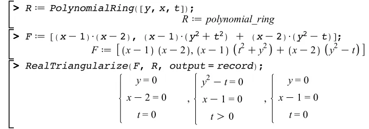
and solve it with theRealTriangularizecommand of theRegularChainslibrary, leading to the computations in Figure 2.3.

> > > >

> >

RdPolynomialRing y,x,t ;

Rdpolynomial_ring

Fd xK1 $ xK2 , xK1 $ y2_C_t2 _C _x_K₂ _$ _y2_K_t _; Fd xK1 xK2 , xK1 t2Cy2 C xK2 y2Kt RealTriangularize F, R, output=record ;

y= 0 xK2 = 0

t= 0 ,

y2Kt= 0 xK1 = 0

tO0 ,

y= 0 xK1 = 0

t= 0

Figure 2.3: A triangular decomposition into semi-algebraic systems computed with the

(38)

BIBLIOGRAPHY 23

The above triangular decomposition consists of three regular semi-algebraic systems.

Let us denote them respectively by [T1, Q1, P1],[T2, Q2, P2],[T3, Q3, P3]. The first and the third ones consist simply of a regular chain, thus we haveP1 =P3 =∅andQ1 =Q3 = true. In fact each of [T1, Q1, P1],[T3, Q3, P3] simply encodes a point, that is, a zero-dimensional component. For the second one, we haveP2 = ∅andQ2 = 0< t, thusT2 = {y2−t, x−1}. Therefore, [T2, Q2, P2], is a parametrization of a one-dimensional component.

> > > > >

> RdPolynomialRing x,y,z ;

Rdpolynomial_ring

Fd 5$x2_C₂_$_z2_$_x_C₅_$_y6_C₁₅_$_y4_K₅_$_y3_K₁₅_$_y5_C₅_$_z2_; Fd 5 y6K15 y5C15 y4C2 z2xK5 y3C5 x2C5 z2 RealTriangularize F,R,output=record ;

5 x2C2 z2xC5 y6C15 y4K5 y3K15 y5C5 z2= 0 25 y6K75 y5C75 y4Kz4K25 y3C25 z2!0 ,

5 xCz2= 0

25 y6K75 y5C75 y4K25 y3Kz4C25 z2= 0 64 z4K1600 z2C25O0

zs0

zK5s0

zC5s0

,

x= 0

yK1 = 0

z= 0 ,

x= 0

y= 0

z= 0 ,

xC5 = 0

yK1 = 0

zK5 = 0 ,

xC5 = 0

y= 0

zK5 = 0 ,

xC5 = 0

yK1 = 0

zC5 = 0 ,

xC5 = 0

y= 0

zC5 = 0 ,

5 xCz2= 0 2 yK1 = 0 64 z4K1600 z2C25 = 0

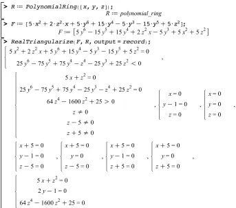
Figure 2.4: Output of the RealTriangularizecommand for the EVEsurface. Figure 2.4 contains a second and more advanced example, where the purpose of the

Maplesession is to obtain a description of the real points of the hypersurfaceEVEfrom the Algebraic Surface Gallery2 and whose equation is 5x2+2xz2+5y6+15y4+5z2−15y5−5y3 = 0. The solutions of the above are all (x,y,z) where x,y,z are complex numbers satisfying this equation. The output of RealTriangularize consists of 9 regular semi-algebraic systems, for which the variables are ordered as x > y > z. The first regular semi-algebraic system represents a two-dimensional component. Indeed, it defines x as the solution of

2_{This is a collection of algebraic surfaces, well-known in the mathematical literature and available at}