Nuclear level density and related physics
VladimirZelevinsky1,∗and SofiaKarampagia2,∗∗
1Department of Physics and Astronomy and National Superconducting Cyclotron Laboratory/Facility for Rare Isotope Beams, Michigan State University, East Lansing, Michigan 48824-1321 USA
2Department of Physics, Grand Valley State University, Allendale, Michigan 49504 USA
Abstract.The knowledge of the level density as a function of excitation energy and nuclear spin is necessary for the description of nuclear reactions and in many applied areas. We discuss the level density problem as a part of the general understanding of mesoscopic systems with strong interactions. The underlying physics is that of quantum chaos and thermalization which allows one to use statistical methods avoiding full diagonalization. The resulting level density is well described by theconstant temperature modelin agreement with experimental data. We discuss the effective temperature parameter and show that it is not related to the pairing phase transition being analogous to the limiting temperature in particle physics. Other aspects of underlying physics include the collective enhancement of the level density, random coupling of individual spins and the role of incoherent collision-like interactions.
1 Introduction
The probabilities of nuclear reactions, including those in atomic industry and in astrophysical conditions, require for their prediction the knowledge of the level density of final nuclei. At energies near the ground state, the levels often can be directly measured. At higher excitation en-ergy, as a rule, there are quite dense sequences of the states with the same exact quantum numbers. In special cases, as reactions induced by slow neutrons of known energy, the individual states can be resolved; in fact here we deal with resonances but in the situation where they do not overlap and can be counted individually.
As discussed in more detail later, with excitation en-ergy growing, the dynamical properties of neighboring states tend to become quite similar due to the strong mix-ing of simple particle-hole configurations by the nucleon interactions. This mixing is getting really strong because of the combinatorial growth of the number of possible el-ementary excitations that unavoidably leads to a dense se-quence of levels. The states with the same total spin J, its projection M, isospin and parity (in a good approxi-mation), starting from a certain excitation energy form a “disordered crystal" [1] with statistical properties locally close to the limit of the Gaussian Orthogonal Ensemble (GOE) which parameters smoothly change along the en-ergy scale. But the random matrix theory does not help in finding the global level density ρ(E) as a function of
excitation energy.
To predict precisely the level density of a complex quantum system, one needs to solve the many-body prob-lem. As this is possible only in very light systems or
∗e-mail: [email protected] ∗∗e-mail: [email protected]
in oversimplified models, the physical approximations are needed. The two main directions are the mean-field meth-ods and configuration interaction approaches. The modern mean-field theory, originated in the Fermi-gas model, is based on the particle-hole combinatorics and includes in some form the pairing interaction [2]. The configuration interaction methods use the matrix diagonalization [3] in a physically truncated orbital space (the shell-models with the currently achievable dimension of the order 1011), the schemes based on the Monte Carlo procedures or statis-tical spectroscopy. We will argue that the statisstatis-tical
mo-ments method [4] is essentially equivalent to full
diago-nalization giving practically exact answers for given space. Both these approaches lose their validity at energy where the states outside the working space appear as intruders. The Monte Carlo techniques [5, 6], as well as mean-field methods, account only for the most regular part of inter-particle interactions, while they do not include incoher-ent collison-like processes which are equally important in forming the realistic level density.
The shell-model calculations taking into account all parts of the interactions show that the typical nuclear level density behaves as in the so-called constant temperature
model (CTM) for energies up to 12-15 MeV (sometimes
even higher) which well describes experimental data. Here
ρ(E)∝exp(E/T) with a constant effective temperature
interpreta-tion [7] in terms of the phase transiinterpreta-tion from the superfluid to normal phase at fixed temperature is not supported by the shell model data.
2 Shell-model level density
The advanced versions of the shell model are defined by a set of single-particle orbitals and matrix elements of all (usually only pairwise) nucleon interactions allowed by the conservation laws. These quantities are determined by comparison of the derived spectroscopic information with the available data. We know that many matrix elements are not uniquely defined by the experiments. However, their presence is important for the correct level density. It is also clear that the shell-model Hamiltonian is not given by a random matrix of uncorrelated elements. Indeed, any two-body process with fixed initial and final orbitals can hap-pen on a different background of other occupancies and therefore the same matrix element repeatedly appears in the Hamiltonian matrix.
In spite of that, the resulting energy spectrum is similar in many respects to the spectra of random matrix ensem-bles [3]. The natural mechanism of this chaotization can be traced through the process of switching on the inter-particle interactions. The eigenstates with the same exact quantum numbers travel through the sequence of multi-ple avoided crossings coming out at the realistic interac-tion strength as extremely complicated superposiinterac-tions of many simple particle-hole configurations. Their mutual repulsion creates the spectral sequences similar to those in the GOE. We come to what can be calledquantum chaos. The global level density is typically given by the Gaus-sian curve with the centroid maximum at energy Em, the
widthσ, and particle-hole symmetry. Although only the
left low part corresponds to realistic physics, the whole curve is instructive as an example of the exact solution of the quantum many-body problem.
Along the level density curve, all observables are ex-pressed as almost unique functions of energy, so that they can be reinterpreted asthermodynamic variables, in spite of absence of an external thermostat. The corresponding thermodynamic temperature is expressed as
Tglobal= σ 2
Em−E; (1)
it is positive on the left branch, jumps from+∞to−∞at the center and becomes negative on the right branch. All observables are smoothly changing along the spectrum as a consequence of the chaotic mixing. This global behavior is in extremely good agreement with the fermionic statis-tics. Namely, we can find, foreach individualeigenstate, occupation numbers of single-particle orbitals. They are well fit by a Fermi-function with certain parameters of temperature and chemical potential. The values of tem-perature found in this way are in perfect agreement with the global temperature (1).
The tails of the Gaussian expression (1), where the chaoticity is not complete, are not fully appropriate at very low (and very high) excitation energy. As many states of
experimental interest are located here, one needs a spe-cial treatment. Phenomenologically, one can use the back-shifted Fermi gas formula [8], where the main energy de-pendence∝exp(√2aE) is defined by the fitted level den-sity parametera. Its value typically is to be taken greater than it would be from the single-particle level density at the Fermi surface; this reflects a stronger energy depen-dence, compare with CTM, Section 4.
3 Moments method
Instead of the diagonalization of extremely large matri-ces, one can successfully use the ideas of statistical spec-troscopy [4, 9] exploiting just the lowest moments of the Hamiltonian. The orbital space is divided intopartitionsp, allowed configurations of particles with certain exact char-acteristicsαand dimensions Dαp. The mean energy of a
partition is defined by the trace
Eαp=Hαp≡ Dα1
pTr
(αp)H. (2)
These centroids form a smooth sequence of mean energies including the interactions inside a partition. The second moment of the Hamiltonian,
H2
αp ≡Dα1
pTr
(αp)H2, (3)
includes the processes of inter-partition interactions. Due to the chaotic nature of the majority of interactions, the contribution of a partition to the many-body level density is very fast converging to a GaussianGαp(E) centered at Eαpof eq. (2) and having a width
σαp=Hα2p−Hαp2. (4)
Finally, the total level density is given by the superposition of those Gaussians,
ρα(E)=
p
DαpGαp(E). (5)
We do not discuss here technical subtleties of this method [4]: the GaussiansGhave a finite range being cut at the edges, because of that they have to be renormalized; energy is counted from the ground state that has to be lo-cated correctly; in an orbital space that includes transitions between oscillator shells, one has to exclude nonphysical admixtures of spurious states related to the center-of-mass motion. There are reliable ways to handle these problems avoiding the huge diagonalization (traces are calculated di-rectly from the matrix ofH). Practically it might be con-venient to use the M-scheme avoiding the heavy algebra of angular momentum. In the majority of cases the M -dependence agrees with what is frequently assumed with the use of a spin-cutoff factor. This supports the idea of random coupling of individual spins (the so-called geo-metric chaoticity); the exceptions are known when spe-cial values of total spin and/or isospin are excluded by the model [10]. The level densityρJ(E) is extracted as a
tion [7] in terms of the phase transition from the superfluid to normal phase at fixed temperature is not supported by the shell model data.
2 Shell-model level density
The advanced versions of the shell model are defined by a set of single-particle orbitals and matrix elements of all (usually only pairwise) nucleon interactions allowed by the conservation laws. These quantities are determined by comparison of the derived spectroscopic information with the available data. We know that many matrix elements are not uniquely defined by the experiments. However, their presence is important for the correct level density. It is also clear that the shell-model Hamiltonian is not given by a random matrix of uncorrelated elements. Indeed, any two-body process with fixed initial and final orbitals can hap-pen on a different background of other occupancies and therefore the same matrix element repeatedly appears in the Hamiltonian matrix.
In spite of that, the resulting energy spectrum is similar in many respects to the spectra of random matrix ensem-bles [3]. The natural mechanism of this chaotization can be traced through the process of switching on the inter-particle interactions. The eigenstates with the same exact quantum numbers travel through the sequence of multi-ple avoided crossings coming out at the realistic interac-tion strength as extremely complicated superposiinterac-tions of many simple particle-hole configurations. Their mutual repulsion creates the spectral sequences similar to those in the GOE. We come to what can be calledquantum chaos. The global level density is typically given by the Gaus-sian curve with the centroid maximum at energy Em, the
widthσ, and particle-hole symmetry. Although only the
left low part corresponds to realistic physics, the whole curve is instructive as an example of the exact solution of the quantum many-body problem.
Along the level density curve, all observables are ex-pressed as almost unique functions of energy, so that they can be reinterpreted asthermodynamic variables, in spite of absence of an external thermostat. The corresponding thermodynamic temperature is expressed as
Tglobal= σ 2
Em−E; (1)
it is positive on the left branch, jumps from+∞to−∞at the center and becomes negative on the right branch. All observables are smoothly changing along the spectrum as a consequence of the chaotic mixing. This global behavior is in extremely good agreement with the fermionic statis-tics. Namely, we can find, foreach individualeigenstate, occupation numbers of single-particle orbitals. They are well fit by a Fermi-function with certain parameters of temperature and chemical potential. The values of tem-perature found in this way are in perfect agreement with the global temperature (1).
The tails of the Gaussian expression (1), where the chaoticity is not complete, are not fully appropriate at very low (and very high) excitation energy. As many states of
experimental interest are located here, one needs a spe-cial treatment. Phenomenologically, one can use the back-shifted Fermi gas formula [8], where the main energy de-pendence∝exp(√2aE) is defined by the fitted level den-sity parametera. Its value typically is to be taken greater than it would be from the single-particle level density at the Fermi surface; this reflects a stronger energy depen-dence, compare with CTM, Section 4.
3 Moments method
Instead of the diagonalization of extremely large matri-ces, one can successfully use the ideas of statistical spec-troscopy [4, 9] exploiting just the lowest moments of the Hamiltonian. The orbital space is divided intopartitionsp, allowed configurations of particles with certain exact char-acteristicsαand dimensions Dαp. The mean energy of a
partition is defined by the trace
Eαp=Hαp≡ Dα1
pTr
(αp)H. (2)
These centroids form a smooth sequence of mean energies including the interactions inside a partition. The second moment of the Hamiltonian,
H2
αp ≡Dα1
pTr
(αp)H2, (3)
includes the processes of inter-partition interactions. Due to the chaotic nature of the majority of interactions, the contribution of a partition to the many-body level density is very fast converging to a GaussianGαp(E) centered at Eαpof eq. (2) and having a width
σαp=Hα2p−Hαp2. (4)
Finally, the total level density is given by the superposition of those Gaussians,
ρα(E)=
p
DαpGαp(E). (5)
We do not discuss here technical subtleties of this method [4]: the GaussiansGhave a finite range being cut at the edges, because of that they have to be renormalized; energy is counted from the ground state that has to be lo-cated correctly; in an orbital space that includes transitions between oscillator shells, one has to exclude nonphysical admixtures of spurious states related to the center-of-mass motion. There are reliable ways to handle these problems avoiding the huge diagonalization (traces are calculated di-rectly from the matrix ofH). Practically it might be con-venient to use the M-scheme avoiding the heavy algebra of angular momentum. In the majority of cases the M -dependence agrees with what is frequently assumed with the use of a spin-cutofffactor. This supports the idea of random coupling of individual spins (the so-called geo-metric chaoticity); the exceptions are known when spe-cial values of total spin and/or isospin are excluded by the model [10]. The level densityρJ(E) is extracted as a
dif-ference ofρM=J−ρM=J+1.
This procedure produces the level densities in various sectors essentially coinciding with the results of the full di-agonalization. Figure 1 compares the shell-model solution and the moment method, the full agreement is obvious. There are small deviations close to the center which can be removed by adding the fourth moment but anyway this region of energy is outside of the physical applicability of the truncated shell model.
0 20 40 60 80 100 0 20 40 60 80 100 120 NLD (MeV -1)
0 20 40 60 80 100 0 50 100 150 200 250
0 20 40 60 80 100 0
100 200 300 400
0 20 40 60 80 100 0 100 200 300 400 500 NLD (MeV -1)
0 20 40 60 80 100 0
100 200 300 400
0 20 40 60 80 100 0
100 200 300 400
0 20 40 60 80 100 0 100 200 300 400 NLD (MeV -1)
0 20 40 60 80 100 0 50 100 150 200 250
0 20 40 60 80 100 0 50 100 150 0 0 20 40 60 80 NLD (MeV -1)
0 20 40 60 80 100 0 10 20 30 40 50
0 20 40 60 80 100 Excitation energy (MeV) 0 5 10 15 20 25
0 20 40 60 80 100 Excitation energy (MeV) 0 2 4 6 8 10 NLD (MeV -1)
0 20 40 60 80 100 Excitation energy (MeV) 0
1 2 3
J=0 J=1 J=2
J=3 J=4 J=5
J=6 J=7 J=8
J=9 J=10 J=11
J=12 J=13
Figure 1. Level densities for various classes of states in thesd shell model of28Si calculated by the full diagonalization (his-tograms) and by the moments method (enveloping lines).
4 Collective enhancement
The configuration interaction approach allows one to study the role of individual matrix elements of the shell-model Hamiltonian looking essentially inside a black box of di-agonalization. It is known that even random interactions respecting the rotational symmetry reproduce some fea-tures of real spectra including the appearance of collective bands. In nuclei, the pairing interaction creates an energy gap for broken pairs. However, there could appear low-lying vibrational states. If the mean field is deformed, many rotational bands appear at low energy. In average, such collective effects increase the level density at low en-ergy [11]. Of course, the total level number in a certain orbital space is fixed.
The shell-model studies confirm the phenomenon of collective enhancement. One way of checking this is based on the earlier results [12] showing the components of the interaction responsible for the nuclear deformation. Us-ing random interactions and findUs-ing the sets of matrix el-ements corresponding to the appearance of the rotational spectrum, it was shown that the main role is played by the processes when one of the particle undergoes a transition with the change of the orbital momentum∆ = ±2 (it is understandable in the spirit of the Nilsson scheme. When
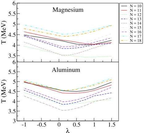
the corresponding matrix elements combined into a part V1 of the Hamiltonian are varied and the interaction pro-duces typical rotational structures, we expect the whole level density curve to shift to low energy. The simplest exercise of this type is illustrated by Figure 2, where the shell-model Hamiltonian is presented as
H=h+λV1+V2, (6)
withhbeing a set of mean-field levels, andV2combining all remaining interaction parts [13, 14].
3.5 4 4.5 5 5.5 6 T (MeV)
N = 10 N = 11 N = 12 N = 13 N = 14 N = 15 N = 16 N = 17 N = 18
-1 -0.5 0 0.5 1 1.5
λ 3 3.5 4 4.5 5 5.5 6 T (MeV) Magnesium Aluminum
Figure 2. The collective enhancement of the low-energy level density for the interaction inducing the rotational spectrum; N gives the neutron number; increase of the effective temperature T corresponds to accumulation of rotational bands at low energy and slower rate of following increase of the level density to its chaotic value, see Refs. [14] and [15].
5 Constant temperature model (CTM)
Currently the most popular phenomenological model of the nuclear level density, suggested long ago by Ericson [16], is expressed asρ(E)=ρ0exp(E/T), (7)
where the normalization factor is usually written asρ0 = (1/T) exp(−E0/T). We can call the main parameterT an
effective temperature. As clear from eq. (7),
1 T = 1 ρ dρ dE (8)
is the rate of the level density growth as a function of en-ergy. The simple parametrization (7) is successfully used by practitioners, including the Oslo group [17].
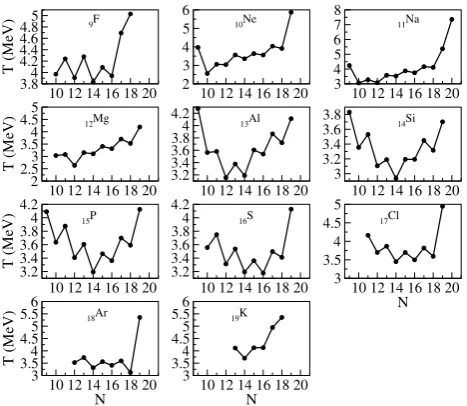
systematically evolves as a function of the isotope com-position, taking minimal values forN = Z in even-even nuclei or in the closest isotopes for odd-Aor odd-odd nu-clei, Figure 4. The partial level density for the sectors with different total spinsJis also well described by the CTM with the slightly varying effective temperature. The com-plete tabulation of the level density parameters for all sd nuclei can be found in Ref. [18].
0 2 4 6 8 10
Excitation Energy (MeV)
0 2 4 6 8
Nuclear level densities (MeV
-1 )
CT, T=2.63, E0=1.49
Moments method
24
Mg
Figure 3.The shell-model level density for thesd-shell nucleus 24Mg, compared to the CTM parametrization.
10 12 14 16 18 20
3.84
4.2 4.4 4.6
4.85
T (MeV)
10 12 14 16 18 20 2
3 4 5 6
10 12 14 16 18 20 3
4 5 6 7 8
10 12 14 16 18 20 2
2.53
3.54
4.55
T (MeV)
10 12 14 16 18 20 3.2
3.4 3.6
3.84
4.2
10 12 14 16 18 20 3
3.2 3.4 3.6 3.8
10 12 14 16 18 20 3.2
3.4 3.6
3.84
4.2
T (MeV)
10 12 14 16 18 20 3.2
3.4 3.6
3.84
4.2
10 12 14 16 18 20 N 3 3.5 4 4.5 5
10 12 14 16 18 20 N 3
3.54
4.55
5.56
T (MeV)
10 12 14 16 18 20 N 3
3.54
4.55
5.56
9F 10Ne 11Na
12Mg 13Al 14Si
15P 16S 17Cl
18Ar 19K
Figure 4.Systematics of the effective temperatureT for the sd-nuclei.Nis the neutron number.
6 Physics of the CTM
Traditionally, the CTM is treated [7] as a realization of a phase transition from superfluid to normal phase of nu-clear matter. In accordance with that, the parameterT is considered as an actual temperature kept constant while the nucleus is heated. The superfluidity is the result of pairing interactions among fermionic quasiparticles. This interpretation contradicts to the shell-model results [13].
Acting similarly to the deformation studies of Section 4, we carefully follow the evolution of the level density as a function of the pairing strength. Here, similarly to eq. (6), we single out the pairing matrix elements,U1, and the rest,
U2,
H=h+k1U1+k2U2. (9) As shown in Figure 5, the effective temperatureT is prac-tically insensitive to the changes of the pairing strengthk1, even with the transition to anti-pairing (k1<0).
2.5 3 3.5 4 4.5
T (MeV)
N = 10 N = 11 N = 12 N = 13 N = 14 N = 15 N = 16 N = 17 N = 18
0 0.2 0.4 0.6 0.8 1 1.2
k
1
3 3.5 4 4.5
T (MeV)
Magnesium
Aluminum
Figure 5.Effective temperatureT and the pairing strengthk1for the isotopes of Mg and Al.Nis the neutron number.
The effective parameter T does not coincide with the thermodynamic temperature Tt−d that can be defined through microcanonical entropy corresponding to the level density (7):
Tt−d(E)=T
1−e−E/T. (10)
This temperature starts from zero at the ground state and grows with energy to its limiting value T. As known from old discussions in particle physics, where the den-sity of resonances is exponentially growing as in the CTM, the limiting temperature signals a gradual transition to the heated chaotic stage. This transition is not directly related to pairing as seen from Figure 5. As was studied earlier [15], the nuclear pairing effects go out with energy through slow crossovers. Another significant check was done with bringing all single-particle energies to degeneracy. Then the CTM description remains valid but the effective tem-perature T goes down. Accordingly, the rate 1/T of in-crease of the level density grows, as expected for easily mixed degenerate mean-field orbitals. The largest rate of chaotization appearing close to the lineN =Zis related to the presence of all isospin values in such nuclei.
systematically evolves as a function of the isotope com-position, taking minimal values forN = Z in even-even nuclei or in the closest isotopes for odd-Aor odd-odd nu-clei, Figure 4. The partial level density for the sectors with different total spinsJis also well described by the CTM with the slightly varying effective temperature. The com-plete tabulation of the level density parameters for all sd nuclei can be found in Ref. [18].
0 2 4 6 8 10
Excitation Energy (MeV)
0 2 4 6 8
Nuclear level densities (MeV
-1 )
CT, T=2.63, E0=1.49
Moments method
24
Mg
Figure 3.The shell-model level density for thesd-shell nucleus 24Mg, compared to the CTM parametrization.
10 12 14 16 18 20
3.84
4.2 4.4 4.6
4.85
T (MeV)
10 12 14 16 18 20 2
3 4 5 6
10 12 14 16 18 20 3
4 5 6 7 8
10 12 14 16 18 20 2
2.53
3.54
4.55
T (MeV)
10 12 14 16 18 20 3.2
3.4 3.6
3.84
4.2
10 12 14 16 18 20 3
3.2 3.4 3.6 3.8
10 12 14 16 18 20 3.2
3.4 3.6
3.84
4.2
T (MeV)
10 12 14 16 18 20 3.2
3.4 3.6
3.84
4.2
10 12 14 16 18 20 N 3 3.5 4 4.5 5
10 12 14 16 18 20 N 3
3.54
4.55
5.56
T (MeV)
10 12 14 16 18 20 N 3
3.54
4.55
5.56
9F 10Ne 11Na
12Mg 13Al 14Si
15P 16S 17Cl
18Ar 19K
Figure 4.Systematics of the effective temperatureT for the sd-nuclei.Nis the neutron number.
6 Physics of the CTM
Traditionally, the CTM is treated [7] as a realization of a phase transition from superfluid to normal phase of nu-clear matter. In accordance with that, the parameterT is considered as an actual temperature kept constant while the nucleus is heated. The superfluidity is the result of pairing interactions among fermionic quasiparticles. This interpretation contradicts to the shell-model results [13].
Acting similarly to the deformation studies of Section 4, we carefully follow the evolution of the level density as a function of the pairing strength. Here, similarly to eq. (6), we single out the pairing matrix elements,U1, and the rest,
U2,
H=h+k1U1+k2U2. (9) As shown in Figure 5, the effective temperatureTis prac-tically insensitive to the changes of the pairing strengthk1, even with the transition to anti-pairing (k1<0).
2.5 3 3.5 4 4.5
T (MeV)
N = 10 N = 11 N = 12 N = 13 N = 14 N = 15 N = 16 N = 17 N = 18
0 0.2 0.4 0.6 0.8 1 1.2
k
1
3 3.5 4 4.5
T (MeV)
Magnesium
Aluminum
Figure 5.Effective temperatureT and the pairing strengthk1for the isotopes of Mg and Al.Nis the neutron number.
The effective parameter T does not coincide with the thermodynamic temperature Tt−d that can be defined through microcanonical entropy corresponding to the level density (7):
Tt−d(E)=T
1−e−E/T. (10)
This temperature starts from zero at the ground state and grows with energy to its limiting value T. As known from old discussions in particle physics, where the den-sity of resonances is exponentially growing as in the CTM, the limiting temperature signals a gradual transition to the heated chaotic stage. This transition is not directly related to pairing as seen from Figure 5. As was studied earlier [15], the nuclear pairing effects go out with energy through slow crossovers. Another significant check was done with bringing all single-particle energies to degeneracy. Then the CTM description remains valid but the effective tem-perature T goes down. Accordingly, the rate 1/T of in-crease of the level density grows, as expected for easily mixed degenerate mean-field orbitals. The largest rate of chaotization appearing close to the lineN=Zis related to the presence of all isospin values in such nuclei.
The exponential regime (7) of the level density cannot continue too far. With onset of quantum chaos, the CTM level density has to match the global Gaussian curve. Near this crossing we should haveTt−d =Tglobal. This is indeed the case as argued in Ref. [19].
7 Role of incoherent interactions
Many developed approaches to the nuclear level density account for the few types of interparticle interactions only. This is natural for theories based on the self-consistent mean field, even with addition of collective modes. Such a limitation is hard to avoid in Monte Carlo approaches due to their notorious sign problem. The shell-model ap-proaches are currently the only ones working with the whole set of interactions. As shown in [10], the pres-ence of incoherent processes (included in termsk2in eq. (9) is necessary in order to obtain the level density as a smooth bell-shape curve; the corresponding contributions are added in quadratures.
In the next development it could be appropriate to sub-stitute the parts of the interaction not defined directly in physical observables by random interactions of suitable strength. Another necessary line of research is the physics of continuum and overlapping resonances.
References
[1] V. Zelevinsky, Annu. Rev. Nucl. Part. Sci.46, 237 (1996)
[2] S. Hillaire, M. Girod, S. Goriely, and A.J. Koning, Phys. Rev. C86, 064317 (2012)
[3] V. Zelevinsky, B.A. Brown, N. Frazier, and M. Horoi, Phys. Rep.276, 85 (1996)
[4] R.A. Sen’kov, M. Horoi, and V. Zelevinsky, Comp. Phys. Comm.184, 215 (2003)
[5] G.H. Lang, C.W. Johnson, S.E. Koonin, and W.E. Or-mand, Phys. Rev. C48, 1518 (1993)
[6] H. Nakada and Y. Alhassid, Phys. Rev. Lett.79, 2939 (1997)
[7] L.G. Moretto, A.C. Larsen, F. Giakoppo, M. Gut-tormsen, and S. Siem, J. Phys. Conf. Series, 580, 012048 (2015)
[8] A. Gilbert and A.G.W. Cameron, Can. J. Phys.43, 1446 (1965)
[9] S.S.M. Wong,Nuclear Statistical Spectroscopy (Ox-ford University Press, 1986)
[10] R. Sen’kov and V. Zelevinsky, Phys. Rev. C 93, 064304 (2016)
[11] A.V. Ignatyuk, K.K. Istekov, and G.N. Smirenkin, Sov. J. Nucl. Phys.29, 450 (1979)
[12] M. Horoi and V. Zelevinsky, Phys. Rev. C81, 034306 (2010)
[13] S. Karampagia and V. Zelevinsky. Phys. Rev. C94, 014321 (2016)
[14] S. Karampagia, A. Renzaglia, and V. Zelevinsky, Nucl. Phys. A962, 46 (2017)
[15] M. Horoi and V. Zelevinsky, Phys. Rev. C75, 054303 (2007)
[16] T. Ericson, Adv. Phys.9, 425 (1960)
[17] M. Guttormsen et al., Phys. Rev. C 89, 014302 (2014)
[18] S. Karampagia, R.A. Sen’kov, and V. Zelevinsky, Atom. Data a& Nucl. Data Tables120, 1 (2018) [19] V. Zelevinsky, S. Karampagia, and A. Berlaga, Phys.