Differential radio map based robust indoor localization

R E S E A R C H

Open Access

Differential radio map-based robust indoor

localization

Jie Wang

, Qinghua Gao

, Hongyu Wang

, Hongyang Chen

and Minglu Jin

Abstract

While wireless local area network-based indoor localization is attractive, the problems concerning how to capture the signal-propagating character in the complex dynamic environment and how to accommodate the receiver gain difference of different mobile devices are challenging. In this article, we solve these problems by modeling them as common mode noise and develop a localization algorithm based on a novel differential radio map approach. We propose a differential operation to improve the performance of the radio map module, where the location is estimated according to the difference of received signal strength (RSS) instead of RSS itself. The particle filter algorithm is adopted to realize the target localization and tracking task. Furthermore, to calculate the particle weight at arbitrary locations, we propose a local linearization technique to realize continuous interpolation of the radio map. The indoor experiment results demonstrate the effectiveness and robustness of our approach.

Keywords:Indoor localization, differential radio map, RSS, particle filter

Introduction

Ubiquitous computing and communication have become popular with the development of wireless communica-tion technology over the last decade. The need for loca-tion informaloca-tion to capture contexts and configure them into the computing and communication processes, coupled with the unavailability of global positioning sys-tem (GPS) in indoor environment, has triggered increased research interest in indoor localization. Recently, numerous localization systems have been developed based on the received signal strength (RSS) of the wireless local area networks (WLANs). The advan-tage of these systems is that the cost of deploying a spe-cialized infrastructure is avoided. However, building an indoor localization system based on WLAN is a challen-ging problem due to the complex indoor signal propaga-tion character and different hardware solupropaga-tions of different mobile devices.

Radio map-based approach is the most widely adopted method to realize indoor localization [1-11]. The essen-tial idea is to construct the radio map by dividing the whole deployment area into cells and then collecting the

RSS measurements from various access points (APs) at each cell, and thus a mobile device can be localized by matching the observed RSS vector with the radio map. In the indoor environment, the RF signal propagation is unpredictable and affected by several factors, such as the presence and movement of human beings, relocation of furniture, multi-path fading, humidity and tempera-ture variations, and closing or opening doors. In such a dynamic environment, the radio map obtained in one time period may not be applicable to other time periods. To solve this problem, Chen et al. [9] built multiple radio maps under various environmental conditions and used sensors to identify the current environment so as to select the most approximate map. Yin et al. [10] off-set the variational environmental factors by adding some reference points as sniffers to capture the dynamic char-acters of the environment and rebuilt the radio map with regression method. Although these methods par-tially overcome the negative effect of dynamic environ-ment, the need for specific infrastructures, such as the environmental sensors and sniffers, makes these meth-ods impractical. More recently, Fang and Lin [11] adopted a temporal sequence of RSS samples as the character vector of the radio map so as to overcome the multipath problem. While this approach demonstrates the effectiveness for the multipath effect, it is of little * Correspondence: [email protected]

1_{Faculty of Electronic Information and Electrical Engineering, Dalian}

University of Technology, No.2 Linggong Road, Ganjingzi District, Dalian, Liaoning Province 116024, People’s Republic of China

Full list of author information is available at the end of the article

use for other problems. The question of how to adapt to the dynamic complex environment without any addi-tional infrastructure is a promising and challenging pro-blem. Because with the changing of environment, it is most likely that the RSS measurements in one location from different APs are prone to shift in the same direc-tion, we can model the dynamic of the indoor environ-ment as the common mode noise. Inspired by the fact that differential signals are widely used in the circuit design to restrain the common mode noise, we adopt the difference of RSS from different APs as the charac-teristic signal of the radio map. Suppose the RSS mea-surement vector from three APs are (RSS1,RSS2, RSS3). Instead of treating it as the fingerprint to realize locali-zation, we adopt the differential vectors (RSS1 - RSS2,

RSS1 - RSS3,RSS2 - RSS3) as fingerprint. Compared with the traditional RSS vector, the differential vector can be effectively adapted to the dynamic indoor environment. Furthermore, it can accommodate the receiver gain dif-ference of different mobile devices. We are aware that the receiver gains of even the same type of devices are different, let alone different types of devices. If the device used in the localization phase is different from that used in the radio map building phase, then the esti-mation error will be increased dramatically. Because the difference of receiver gain offsets the RSS measurements in the same direction, we can also model it as common mode noise.

In this article, we propose a novel robust indoor loca-lization algorithm under the framework of Bayesian fil-ter. The particle filter (PF) [12,13] is adopted to achieve the localization and tracking task, which makes full use of the history observation to improve the estimation accuracy. The differential radio map is used for building the observation likelihood for the PF algorithm so as to solve the dynamic environment and different receiver gain problem. For the sake of predicting signal strength measurements at arbitrary locations so as to calculate particle weight and improve localization accuracy, we also adopt a local linearization technique to realize con-tinuous interpolation of the radio map.

This article is organized as follows. Section II provides a brief overview of the indoor localization problem. In Section III, the definition of the differential radio map is given, and the localization architecture is described from the view of system. The detailed implementation of our differential radio map-based PF algorithm is presented in Section IV. Section V validates our algorithm by eva-luations. Finally, the conclusion is drawn in Section VI.

Related works

Indoor localization with WLAN has been an active research area in the last decade. Honkavirta et al. [14] presented a survey of location fingerprinting methods,

and Seco et al. [15] reviewed the indoor localization algorithms from the aspect of mathematic. In this sec-tion, we give a brief overview of some key research find-ings in this area. Considering the needs of building the radio map, we divide the methods into map-based and non-map based algorithms.

radio map to make the algorithm more robust and a local linearization technique to realize continuous inter-polation of the radio map.

Besides the above research studies, some schemes based on the deterministic and proba-bilistic framework have also been developed. Lim et al. [16] used the trun-cated singular value decomposition to calculate the sig-nal-distance map (SDM) based on the online measurements between the APs. Although the dynamic SDM makes it possible to capture the challenging dynamic indoor environment, the requirements of the high AP density and the modification of commercial AP’s software make the scheme impractical. Hossain et al. [17] proposed a robust localization algorithm that could make use of multiple wireless techniques. Schwaighofer et al. [18] first adopted the Gaussian pro-cess (GP) as a non-parametric tool to realize the approximation of the radio map of cellular network. Fer-ris et al. [19] introduced the GP into the WLAN-based indoor localization. Compared with other regression models, the GP takes into account the noise of the observation and provides the ability to approximate nonlinear signal propagation model. Madigan et al. [20] adopted a Bayesian hierarchical approach to realize indoor localization, which eliminated the need of know-ing the locations of the trainknow-ing points. Huang et al. [21] proposed a similar Bayesian algorithm and intro-duced the stochastic properties of measurement errors and the reliability of the measurement data into the fac-tor graph framework so as to improve the accuracy. Wymeersch et al. [22] also proposed a Bayesian localiza-tion algorithm and took the cooperalocaliza-tion of the nodes into consideration to improve the accuracy. Feng et al. [23] employed the compressive sensing theory to analyze the localization problem. The localization problem is modeled as a sparse question and can be solved by the L1 minimization. While these methods cut down the measurement effort and partially adapt to the dynamic environment, they still require effort in terms of placing sniffers, modifying commercial AP’s software, obtaining the knowledge of AP placement, and of complex computation.

Differential radio map and system architecture In this section, we define the differential radio map and analyze its ability to restrain the dynamic environmental noise and receiver gain difference. The architecture of the proposed localization system is presented thereafter.

Differential radio map

The construction of the differential radio map is almost the same as that of the traditional radio map, except that a differential operation module is introduced. First, we divide the deployment area into equal square

training cells with their vertices set as the training points. Then, we perform off-line training to record RSS measurements transmitted by each AP and store these measurements into the radio map. The radio map has the following form:

Map ={pi, Ri|i = 1, . . ., M},Ri={Rij|j∈Ni}, (1)

whereMis the total number of training points, piand

Riindicate the location and fingerprint of the ith train-ing point, respectively,Ni is the detected AP list at the

ith training point, Rijis a Gaussian PDF represented by

N(μij, σ_ij2)with the meanμij, and covarianceσij2, which

is used to approximate the RSS measurements collected at theith training point and transmitted by thejth AP.

Unlike the traditional radio map which adopts the fin-gerprintRidirectly for localization, we adopt the differ-ential fingerprintR¯iwhich takes theRias input, and it is calculated as follows:

¯

Ri={Rij−Rim|j∈Ni, j= m}, Rim= max{Rij|j∈Ni}, (2)

where Rim is the strongest RSS measured at the ith

training point (the measurement with lower ID is adopted when equal RSSs are measured), andRij-Rimis represented byN(μij−μim,σ_ij2+σ_im2).

In theory, the propagation of radio signal is regulated by a certain principle. The shadowing model is widely adopted to approximate the signal propagation character

in the indoor circumstance. With this model, Rij is

defined by

Rij=G+Pj−Lj−10βlog10dij+v, (3)

where Gis the receiver gain, Pj is the transmitting power (dBm) of the jth AP,Lj is the signal attenuation power (dBm) at the distance of 1 m,b is the path loss exponent,dijis the Euclidean distance between the ith training point andjth AP, andvrepresents the

measure-ment noise. G+ Pj - Lj is always represented by one

symbol and is called the received power at the distance of 1 m in other studies. To analyze the feature of the differential operation, we use three symbols to represent each factor here. The dynamic indoor environment

always causes the change of parameters Ljand b, and

the change of these parameters incur the change of the

Rij.As for different types of device, the receiver gainG is different, and thus the change of device causes the change ofRij, as well.

The differential RSS is calculated as

Rij−Rim= (Pj−Pm)−(Lj−Lm)−10β(log10dij−log10dim) +˜v, (4)

where Pj - Pm is a constant which does not change

with environment. While Lj and Lm change with the

Consequently, the change of Lj-Lm is not significant

compared with the change of Lj and Lm. As for 10b

(log10 dij - log10 dim), since log10 dij - log10 dim is less than log10dijand log10dim, the change must be insignif-icant, too. From Equation 4, we can see that the termG

is eliminated in the expression. Therefore, the differen-tial RSS scheme is immune to the dynamic indoor envir-onment, and can solve the problem caused by different receiver gains of multi-devices.

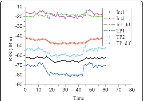
To validate the above theoretical analysis, we placed two different types of mobile devices at the same loca-tion and collected RSS measurements from two APs located at different places. We used an Intel 4965AGN wireless card and a TP-LINK TL-WN322G wireless card to gather RSS. There is a door between the wireless cards and APs, and we closed the door in the time instant 15-45. We define Int1 and Int2 as the RSS mea-surements, respectively, from AP1 and AP2 by 4965AGN, TP1 and TP2 as the RSS measurements by TL-WN322G, Int_dif as the differential signal of Int1 and Int2, and TP_dif as the differential signal of TP1 and TP2. Figure 1 demonstrates that the change of the differential RSS is quite insignificant compared with the change of RSS. It can also be seen that while the differ-ence of the RSS measurements from the same AP with different devices is remarkable, the difference of differ-ential RSS measurements is almost the same. The aver-age differences between Int1 and TP1, Int2 and TP2 are 10.5 and 11.3, respectively, while that between Int_dif and TP_dif is only 0.8.

System architecture

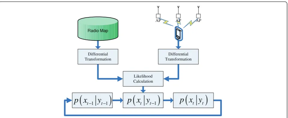
The system flow of the proposed differential radio map-based localization system is plotted in Figure 2, wherext is the current estimated location information, ytis the current observation, p(xt-1 |yt-1) is the posterior PDF

estimation of time instantt -1,p(xt|yt-1) andp(xt|yt) are the prior and posterior PDF estimations of time instantt, respectively.

The localization system follows the framework of Bayesian filter [12,13] and estimates the posterior PDF of the location recursively conditioned on all the mea-surements,y1,...,yt. The essential of the Bayesian filter is the prediction process and observation update process, which are defined as follows:

p(xt|yt−1) = model, which describes the motion of the mobile device, and p (yt|xt) represents the observation likelihood model, which describes the likelihood of observing a dif-ferential RSS measurement vectorytat a locationxt. We describe the detailed models in the next section.

Implementation of the algorithm

This section first gives a brief introduction of the PF algorithm, and then defines the motion model and observation model in detail.

PF algorithm for localization and tracking

Bayesian filter algorithms [24] have achieved great suc-cess in handling the localization and tracking problem through the sequential estimation of target’s state, coop-eration with the movement modeling, prior distribution prediction, and posterior distribution estimation. Among these Bayesian filter algorithms, the PF algorithm [12,13] has emerged as a popular choice because of its unique ability in dealing with the complex non-Linear and non-Gaussian estimation problem. For these rea-sons, we adopt the PF algorithm for localization in this article. The PF algorithm approximates the probability distribution of the estimated target with several weighted particles, and deals with the sequential estima-tion by carrying out a series of particle-propagating operations. Let _{xi

t, wit|i= 1, . . ., N}denote a particle

set, wherexit is a sample ofxtwith associated normal-ized weightwi

where δ () is the Dirac delta function. Suppose we

have the proposal distribution q (xt|xt-1, yt), then the

predicted location xi_t can be generated based on the

0 10 20 30 40 50 60 70 80

previous location xi

Most articles in the literature define the proposal dis-tribution asq(xt|xt-1,yt) =p(xt|xt-1), which only consid-ers the motion model and neglects the latest observation

yt. For simplicity, we follow this scheme. Interested readers could find out the methods of designing advanced proposal distribution in [25]. Now, the ques-tion is how to define the moques-tion model p(xi

t|xit−1)and

the observation likelihood model p(yt|xit) for the

particles.

Motion model

Speaking in general, the motion model of the mobile devices in the indoor environment is untraceable, and the velocity and direction of the mobile device are hard to estimate. In [19], Ferris et al. used a voronoi graph to aid the motion prediction. Although the performance of the prediction is improved, it needs detailed floor plan of the building which is impractical and inconvenient. Jin et al. [26] adopted dead reckoning sensors to make prediction, which needs the additional expensive sen-sors. Based on the principle of making the system as universal as possible, we define the motion model purely based on the historical motion information. We consider only two-dimensional localization, and the extension to the three-dimensional scenario is straightforward. The

two-dimensional location statextcan be represented by (Xt, Yt). Suppose the location states of the previous two time instants are,xt-2and xt-1, the predicted velocityvˆt

and directionαt of the mobile device can be estimated

as follows:

where vmax is the velocity threshold of the mobile

device and generally set as 1m/s. The motion model of the particles can be written as

cles are generated in the fan-shaped area. Meanwhile, to cope with the circumstance such as the swerve of the mobile device, we randomly select 80% particles that participate in the prediction defined by Equation 12, and let the rest 20% particles randomly move in the cir-cular area, with the last estimation as center andvmax as radius.

Observation likelihood model

In order to calculate the likelihood of the particles at arbitrary locations, the first thing that should be solved is to fulfill the radio map with the ability of representing the RSS measurements at arbitrary locations. The radio map defined by Equation 1 is a discrete map, and only Radio Map

the RSS fingerprints of the training points are recorded. We adopt a linearization technique to predict RSS mea-surements at arbitrary locations. Within each of the square training cells, we use a hyperplane to approxi-mate the RSS measurements of every AP. The 3D plane equation includes (x, y, r) coordinate, where (x, y) is the

2D location, andr is RSS measurement. The equation is

defined as

a

×

x

+

a

×

y

+

a

×

r

=

c

,

whereax, ay, andarare the coefficients of the plane

equation, andc is a non-zero constant and set as 1 in

this article. The RSS measurements of the four vertices and their locations are known, therefore, they can be used to calculate the coefficients of the hyperplane equation. Suppose the locations of the four vertices are (x1,y1), (x2,y2), (x3, y3), and (x4,y4), the mean values of the RSS measurements from one AP are r1, r2,r3, and

r4. We have a constraint matrix in the following form:

A·B=C, (14)

The coefficients of the hyperplane equation can be

solved with the least square algorithm as

B=AT_A−1_AT_{C, where ()}-1

and ()Trepresent the matrix inverse and transpose, respectively. After building the hyperplane equation for every AP in each of the square training cells, the mean value of RSS fingerprint at an arbitrary location can be calculated with Equation 13, and the average value of the four vertices’covariance is set as the covariance of the location.

For the particlexi

t, we first judge which training cell it

belongs to and calculate the RSS fingerprint vector based on the hyperplane equation, and then, we trans-form the RSS fingerprint vector and the current, observed RSS measurement vector to their differential form. Suppose the differential fingerprint for thejth AP is N(μ¯ij, σ¯_ij2), the observed differential RSS

measure-ment from the jth AP iso¯j, then the likelihood for the jth AP is N(o¯j;μ¯ij, σ¯_ij2). Suppose the RSS measurements

from different APs are independent, the observation likelihood can be expressed as

p(yt|xit) =

wherenis the number of detected APs. The exponent

1/nis used to smooth the likelihood so as to avoid the occurring of overconfident estimate. We calculate the observation likelihood values for all the particles and adopt wi_t−1p(yt|xit)as the new particle weight, and then,

normalize it to ensure the summation of weights is equal to 1.

With the normalized weighted particle set

{xit,wit|i= 1,. . .,N}, the location estimation xt can be

degeneration problem, we adopt the adaptive systematic resample method [25] for further optimizing the quality of the particles. The outline of our differential radio map-based Bayesian localization (DRMBL) algorithm is summarized in Table 1.

Experimental evaluation

In this section, we start by giving a detailed presentation of our testbed. Then, we evaluate the proposed improve-ment strategies under different conditions. For simplicity and comparison, the deterministic fingerprint-based

RADAR algorithm adopts the weightedk-nearest

neigh-bor technique, abbreviated as KNN, and the algorithm that adopts probabilistic fingerprint localization techni-que is abbreviated as PL. Furthermore, to evaluate the effectiveness of our differential strategy, the differential strategy is also applied to the KNN and PL algorithms. We define the improved algorithms as DRMKNN and DRMPL, respectively.

Experiment setup

To evaluate the performance of our algorithm, we per-formed realistic experiment on the second floor of the Electronic Information building of Dalian University of

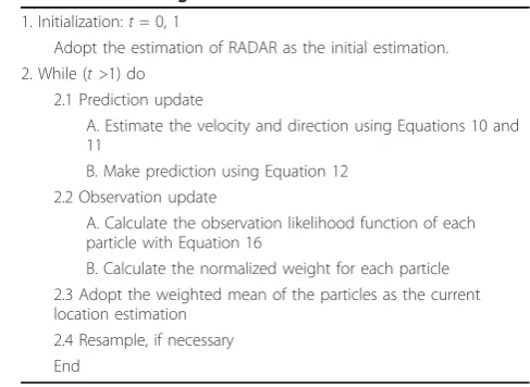
Table 1 DRMBL algorithm

1. Initialization:t= 0, 1

Adopt the estimation of RADAR as the initial estimation. 2. While (t >1) do

2.1 Prediction update

A. Estimate the velocity and direction using Equations 10 and 11

B. Make prediction using Equation 12 2.2 Observation update

A. Calculate the observation likelihood function of each particle with Equation 16

B. Calculate the normalized weight for each particle 2.3 Adopt the weighted mean of the particles as the current location estimation

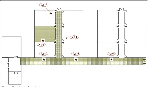
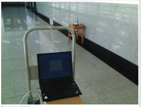
Technology. The layout of the floor is shown in Figure 3, and a scene of training is illustrated in Figure 4. The

deployment area has a dimension of 72 ×29 meters.

The TP-LINK TL-WR340G+ APs are adopted, and there

are six detectable APs on the floor. We use an IBM ThinkPad X60 laptop with Windows XP operating sys-tem as the mobile device. A TP-LINK TL-WN322G wireless card is adopted to gather RSS in the radio map building phase, and a 4965AGN card and a TL-WN322G wireless card are used in the localization phase. Unless otherwise specified, we adopted the data collected by 4965AGN in the following evaluations. We designed the software for collecting RSS based on the NDIS Miniport [27].

The radio map has 164 locations along the corridor and 70 locations inside the room. We placed the train-ing points 1.2 m apart and collected 10 samples at each point with a time interval of 1 s. The default parameters

for the algorithms are as follows: the parameter kof

KNN is 4, and the number of particles used in the DRMBL is 1000.

Evaluation results

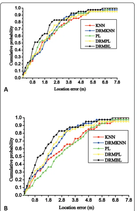
Figure 5a demonstrates the comparison of the cumula-tive distribution function (CDF) of the localization error when using a TL-WN322G wireless card which is the same as that used in the training phase; the DRMBL algorithm outperforms other algorithms and its average

localization error decreases by 13% compared with KNN. The average localization errors of DRMKNN and DRMPL algorithms decrease by 4% and 3.7%, respec-tively, when comparing with KNN and PL algorithms. Figure 5b shows the localization error when using an Intel 4965AGN wireless card. It can be seen that the performances of DRMBL, DRMKNN, and DRMPL algo-rithms are nearly the same as that of Figure 5a, while the performance of KNN and PL algorithms drops dra-matically. These results show the effectiveness of our improvement strategies, and indicate that the differential method is generic and can be applied to other localiza-tion algorithms to improve their accuracy.

Table 2 summarizes the detailed results. It can be seen that comparing with KNN and PL algorithms, the aver-age error of DRMBL decreases by more than 26% and 22%, respectively. With our differential strategy, the average errors of DRMKNN and DRMPL decrease by more than 18% and 10%. However, it should be men-tioned that the maximum errors of DRMKNN and DRMPL increases, respectively, by 35% and 36%. This is because when the RSS measurements from the reference AP incur from severe noise, the differential operation may bring noise to the differential RSS vector, which incurs the increase of localization error. Hence, the selection of reference AP is of vital importance.

To evaluate the performance of our DRMBL algorithm under different conditions, we studied the sensitivity of

AP4

AP3

AP2

AP1

AP5

AP6

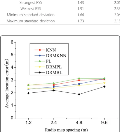
the algorithm to the number of APs and radio map spa-cing. Figure 6a illustrates that the average localization error decreases gradually with the increase of the num-ber of APs, and a relatively stable condition can be achieved when the number of APs is greater than 4. In Figure 6b, the error bars represent the standard devia-tion. It demonstrates nearly the same character as that of average error. It can be seen from Figure 7 that the accuracy decreases and standard deviation increases gra-dually with the increase of radio map spacing. However, the DRMBL algorithm still achieves average error of 2.56 m at the radio map spacing of 9.6 m. It can be learned from Figure 7a that the performances of DRMKNN and DRMPL drop dramatically with the increase of radio map spacing; because with the decrease of the number of training points, the RSS measurement from the reference AP may be far away from any train-ing points, which introduces noise to the differential RSS vector.

Essentially speaking, our DRMBL algorithm is a PF algorithm, and the performance of PF algorithm

depends largely on the number of particles adopted in the algorithm. We evaluated the algorithm using differ-ent number of particles. Figure 8 illustrates that with the increase of the number of particles, the average error and its standard deviation decrease gradually. It can be seen that 100 particles are sufficient for the algo-rithm to achieve reasonable results.

Figure 9 demonstrates the tracking effect of our DRMBL algorithm. A mobile device is moving in the deployment area, its motion trace covers straight corri-dor with excellent AP signal coverage and corner with noisy and feeble AP signal. In Figure 9a, the blue “L” shape line is the ground truth trace, and the black trace is the estimated one. We can see that, in the corridor, the tracking performance is very good; however, in the corner, the estimation error increases remarkably. For clarity, we mark the poor estimations with red stars and plot the detailed estimation errors in Figure 9b. From Figure 9, we can learn that one should pay special atten-tion to the placement of APs to ensure that the radio signal could cover every corner in the deployment area.

Discussion

We highlight some of the experience on the DRMBL algorithm, including the differential strategy, the density of training points, and the characteristic of the PF algorithm.

It should be mentioned that the differential strategy is generic. It can be adopted by any localization system as long as they use the RSS as measurement, such as WLAN, Zigbee, Bluetooth, and GSM-based systems. If

NAPs are detected, ideally there areC2

N pairs of

differ-ential RSS measurements. For simplicity, we select the

AP with the strongest RSS as the reference AP and select N -1 differential RSS measurements relative to it according to Equation 2. Computational resources per-mitting, one can utilize all the differential measurements to improve the performance. The performance of the differential strategy is greatly affected by the reference AP. Therefore, the selection of the most appropriate reference AP is vital for the DRMBL algorithm. We have verified four criteria: AP with the strongest RSS, AP with the weakest RSS, AP with the minimum stan-dard deviation, and AP with the maximum stanstan-dard deviation. Table 3 illustrates that the criterion of select-ing the AP with the strongest RSS is superior to others.

As has been seen from Figure 7a, one shortcoming of the differential strategy is that it requires dense training points. Our DRMBL algorithm solves this problem with continuous interpolation technique. When the differen-tial strategy is adopted, we suggest that the interpolation technique could be used for generating some virtual training points. Figure 10 demonstrates the results of

Table 2 Comparison of localization error

Algorithm Median (m)

Average (m)

Stand deviation (m)

90% (m)

Max (m)

KNN 2.42 2.78 1.89 5.28 7.34

DRMKNN 1.97 2.28 1.85 4.19 9.95

PL 2.26 2.60 1.86 4.82 7.50

DRMPL 1.92 2.34 2.12 4.61 10.23

DRMBL 1.49 2.04 1.75 4.17 6.80

A

B

Figure 5CDF of localization error with different hardware.

A

B

DRMKNN and DRMPL with interpolation technique used in the radio maps of 4.8 and 9.6 m spacings.

Moreover, with the essential similarity to PF algorithm, DRMBL deals with the location estimation problem by means of prediction and observation update process. In this article, we suppose that the algorithm knows nothing about the prior knowledge; if we have some prior infor-mation about the velocity or direction, the tracking accu-racy will be improved significantly. Figure 11 demonstrates the localization error for tracking the same trace as that of Figure 9a while having prior velocity information. The estimation error is remarkably reduced, and the average localization error is only 1.17 m.

Conclusion

To address the problem of realizing accurate localization in complex dynamic environment in the WLAN which

A

B

Figure 7Impact of the radio map spacing.

Figure 8Impact of the number of particles.

A

B

is made up of different types of devices, we proposed a novel DRMBL algorithm under the Bayesian framework. We proposed a differential strategy to overcome the common mode noise and a continuous interpolation technique to accurately realize the particle weight calcu-lation. The experiments validated our proposed schemes, and revealed that DRMBL algorithm could

achieve reasonable localization results under challenging background conditions. The schemes proposed in this article are generic and could be adopted by other locali-zation systems.

Abbreviations

CDF: cumulative distribution function; DRMBL: differential radio map-based Bayesian localization; GPS: global positioning system; PDF: probability distribution function; RSS: received signal strength; SDM: signal-distance map; WLAN: wireless local area network.

Acknowledgements

This study was supported by the National Natural Science Foundation of China under grant numbers 60871046 and the National Hi_Tech Research and Development 863 program of China under grant numbers 2008AA092701. The authors thank the constructive discussions with their group members during the writing of the article. The authors would also like to thank the reviewers for their useful suggestions and comments.

Author details

1_{Faculty of Electronic Information and Electrical Engineering, Dalian}

University of Technology, No.2 Linggong Road, Ganjingzi District, Dalian, Liaoning Province 116024, People_’s Republic of China2_{Institute of Industrial}

Science, The University of Tokyo, Tokyo, Japan

Competing interests

The authors declare that they have no competing interests.

Received: 24 November 2010 Accepted: 16 June 2011 Published: 16 June 2011

References

1. P Bahl, VN Padmanabhan, RADAR: an in-building RF-based user location and tracking system, inProceedings of the 19th IEEE International Conference on Computer Communications (INFOCOM‘00),vol. 2, (Tel Aviv, Israel, March 2000), pp. 775–784

2. TP Deasy, WG Scanlon, Simulation or measurement: the effect of radio map creation on indoor WLAN-based localisation accuracy. Wirel Personal Commun,42(4), 563–573 (2007)

3. TC Tsai, CL Li, TM Lin, Reducing calibration effort for WLAN location and tracking system using segment technique, inProceedings of the IEEE International Conference on Sensor Networks, Ubiquitous, and Trustworthy Computing (SUTC‘06),vol. 2, (Taichung, Taiwan, June 2006), pp. 46–51 4. XY Chai, Q Yang, Reducing the calibration effort for probabilistic indoor

location estimation. IEEE Trans Mobile Comput,6(6), 649–662 (2007) 5. B Philipp, Redpin–adaptive, zero-configuration indoor localization through

user collaboration, inProceedings of the 1st ACM international workshop on Mobile entity localization and tracking in GPS-less environments (MELT‘08)

(San Francisco, USA, September 2008), pp. 55–60

6. K Chintalapudi, AP Iyer, VN Padmanabhan, Indoor localization without the pain, inProceedings of the 16th Annual International Conference on Mobile Computing and Networking (MOBICOM‘10)(Chicago, USA, September 2010), pp. 173_–184

7. Y Wu, JB Hu, Z Chen, Radio map filter for sensor network indoor localization systems, inProceedings of the 5th IEEE International Conference on Industrial Informatics (INDIN‘07)(Vienna, Austria, July 2007), pp. 63–68 8. M Youssef, A Agrawala, The Horus location determination system. Wirel

Netw,14(3), 357–374 (2008)

Table 3 Comparison of the reference AP selection criterions

criterion Median (m) Average (m) Stand deviation (m) 90% (m) Max (m)

Strongest RSS 1.43 2.01 1.71 4.27 6.80

Weakest RSS 1.91 2.36 1.71 4.72 7.16

Minimum standard deviation 1.66 2.06 1.64 4.12 7.13

Maximum standard deviation 1.73 2.18 1.79 4.32 8.08

Figure 10Impact of the radio map spacing with interpolation.

9. YC Chen, JR Chiang, HH Chu, P Huang, AW Tsui, Sensor-assisted wi-fi indoor location system for adapting to environmental dynamics, in

Proceedings of the 8th ACM international symposium on Modeling, analysis and simulation of wireless and mobile systems (MSWiM_‘05)(Montreal, Canada, October 2005), pp. 118–125

10. J Yin, Q Yang, LM Ni, Learning adaptive temporal radio maps for signal-strength-based location estimation. IEEE Trans Mobile Comput,7(7), 869_–883 (2008)

11. SH Fang, TN Lin, A dynamic system approach for radio location fingerprinting in wireless local area networks. IEEE Trans Commun,58(4), 1020–1025 (2010)

12. A Doucet, S Godsill, C Andrieu, On sequential Monte Carlo sampling methods for Bayesian filtering. Stat Comput,10(3), 197_–208 (2000) 13. PM Djuric, JH Kotecha, JQ Zhang, YF Huang, T Ghirmai, MF Bugallo,

J Miguez, Particle filtering. IEEE Signal Process Mag,20(5), 19_–38 (2003) 14. V Honkavirta, T Perala, S Ali-Loytty, R Piche, A comparative survey of WLAN

location fingerprinting methods, inProceedings of the 6th Workshop on Positioning, Navigation and Communication (WPNC‘09)(Hannover, Germany, March 2009), pp. 243–251

15. F Seco, AR Jimenez, C Prieto, J Roa, K Koutsou, A survey of mathematical methods for indoor localization, inProceedings of the 6th IEEE International Symposium on Intelligent Signal Processing (WISP_‘09)(Budapest, Hungary, August 2009), pp. 9–14

16. H Lim, LC Kung, JC Hou, HY Luo, Zero-configuration, robust indoor localization: theory and experimentation, inProceedings of the 25th IEEE International Conference on Computer Communications (INFOCOM_‘06)

(Barcelona, Spain, April 2006), pp. 1–12

17. M Hossain, HN Van, Y Jin, WS Soh, Indoor localization using multiple wireless technologies, inProceedings of the 4th IEEE International Conference on Mobile Adhoc and Sensor Systems (MASS‘07)(Pisa, Italy, October 2006), pp. 1–8

18. A Schwaighofer, M Grigoras, V Tresp, C Hoffmann, GPPS: a Gaussian process positioning system for cellular networks, inProceedings of the 7th Conference on Neural Information Processing Systems (NIPS‘03)(Whistler, Canada, December 2003), pp. 1_–8

19. B Ferris, D Hahnel, D Fox, Gaussian processes for signal strength-based location estimation, inProceedings of the 2nd Robotics: Science and Systems (RSS‘06)(Philadelphia, USA, August 2006), pp. 1–8

20. D Madigan, E Einahrawy, RP Martin, WH Ju, P Krishnan, AS Krishnakumar, Bayesian indoor positioning systems, inProceedings of the 24th IEEE International Conference on Computer Communications (INFOCOM‘05),vol. 2, (Miami, USA, March 2005), pp. 1217_–1227

21. CT Huang, CH Wu, YN Lee, JT Chen, A novel indoor RSS-based position location algorithm using factor graphs. IEEE Trans Wirel Commun,8(6), 3050–3058 (2009)

22. H Wymeersch, J Lien, MZ Win, Cooperative localization in wireless networks. Proc IEEE,97(2), 427–450 (2009)

23. C Feng, WSA Au, S Valaee, ZH Tan, Compressive sensing based positioning using RSS of WLAN access points, inProceedings of the 29th IEEE International Conference on Computer Communications (INFOCOM‘10)(San Diego, USA, March 2010), pp. 1631–1639

24. D Fox, J Hightower, L Lin, D Schulz, G Borriello, Bayesian filtering for location estimation. IEEE Pervas Comput,2(3), 24_–33 (2003)

25. AM Johansen, A Doucet, A note on auxiliary particle filters. Stat Probab Lett, 78(12), 1498_–1504 (2008)

26. YY Jin, M Motani, WS Soh, JJ Zhang, SparseTrack: enhancing indoor pedestrian tracking with sparse infrastructure support, inProceedings of the 29th IEEE International Conference on Computer Communications (INFOCOM ‘10)(San Diego, USA, March 2010), pp. 668–676

27. The Code Project. http://www.codeproject.com/KB/IP/wlanscan_ndis.aspx

doi:10.1186/1687-1499-2011-17

Cite this article as:Wanget al.:Differential radio map-based robust indoor localization.EURASIP Journal on Wireless Communications and Networking20112011:17.

Submit your manuscript to a

journal and benefi t from:

7 Convenient online submission

7 Rigorous peer review

7 Immediate publication on acceptance

7 Open access: articles freely available online

7 High visibility within the fi eld

7 Retaining the copyright to your article