Volume 2010, Article ID 192752,12pages doi:10.1155/2010/192752
Research Article
ε
-Net Approach to Sensor
k
-Coverage
Giordano Fusco and Himanshu Gupta
Computer Science Department, Stony Brook University, Stony Brook, NY 11790, USA
Correspondence should be addressed to Giordano Fusco,[email protected]
Received 31 August 2009; Accepted 10 September 2009 Academic Editor: Benyuan Liu
Copyright © 2010 G. Fusco and H. Gupta. This is an open access article distributed under the Creative Commons Attribution License, which permits unrestricted use, distribution, and reproduction in any medium, provided the original work is properly cited.
Wireless sensors rely on battery power, and in many applications it is difficult or prohibitive to replace them. Hence, in order to prolongate the system’s lifetime, some sensors can be kept inactive while others perform all the tasks. In this paper, we study the
k-coverage problem of activating the minimum number of sensors to ensure that every point in the area is covered by at least
ksensors. This ensures higher fault tolerance, robustness, and improves many operations, among which position detection and intrusion detection. Thek-coverage problem is trivially NP-complete, and hence we can only provide approximation algorithms. In this paper, we present an algorithm based on an extension of the classicalε-net technique. This method gives anO(logM )-approximation, whereMis the number of sensors in an optimal solution. We do not make any particular assumption on the shape of the areas covered by each sensor, besides that they must be closed, connected, and without holes.
1. Introduction
Coverage problems have been extensively studied in the context of sensor networks (see, e.g., [1–4]). The objective of sensor coverage problems is to minimize the number of active sensors, to conserve energy usage, while ensuring that the required region is sufficiently monitored by the active sensors. In an over-deployed network we can also seekk-coverage, in which every point in the area is covered by at least k sensors. This ensures higher fault tolerance, robustness, and improves many operations, among which position detection and intrusion detection.
The k-coverage problem is trivially NP-complete, and hence we focus on designing approximation algorithms. In this paper, we extend the well-known ε-net technique to our problem and present anO(logM)-factor approximation algorithm, where M is the size of the optimal solution. The classical greedy algorithm for set cover [5], when applied tok-coverage, delivers anO(klogn)-approximation solution, where n is the number of target points to be covered. Our approximation algorithm is an improvement over the greedy algorithm, since our approximation factor of O(logM) is independent ofk and of the number of target points.
Instead of solving the sensor’s k-coverage problem directly, we consider a dual problem, the k-hitting set. In the k-hitting set problem, we are given sets and points, and we look for the minimum number of points that “hit” each set at least k times (a set is hit by a point if it contains it). Br¨onnimann and Goodrich were the first [6] to solve the hitting set using the ε-net technique [7]. In this paper, we introduce a generalization of ε-nets, which we call (k,ε)-nets. Using (k,ε)-nets with the Br¨onnimann and Goodrich algorithm’s [6], we can solve the k-hitting set, and hence the sensor’sk-coverage problem. Our main contribution is a way of constructing (k,ε)-nets by random sampling. A recent Infocom paper [8] uses ε-nets to solve the k-coverage problem. However we believe that their result is fundamentally flawed (see Section 2.1 for more details). So, to the best of our knowledge, we are the first to give a correct extension of ε-nets for the k-coverage problem.
Paper Organization. The rest of the paper is organized as follow. Thek-coverage problem is introduced inSection 2.
∗s1
(a)
∗s2
(b)
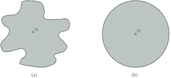
Figure1: Sensing regions associated with a sensor: (a) a general shape that is closed, connected, and without holes, and (b) a disk.
∗s1 ∗
s2
∗s4 ∗s3
(a)
∗s1 ∗
s2
∗s4 ∗s3
(b)
Figure2: Illustratingk-SC problem. Suppose we are given 4 sensors of centerss1,. . .,s4and 20 points as in (a). The problem is to select the
minimum number of sensors tok-cover all points. A possible solution fork=2 is shown in (b), where 3 sensors suffice to 2-cover all points.
2. Problem Formulation and Related Work
We start by defining the sensing region and then we will define thek-coverage problem with sensors. In the literature, sensing regions have been often modeled as disks. In this paper, we consider sensing regions of general shape, because this reflects a more realistic scenario.
Definition 1(sensing region). The sensing region of a sensor is the area “covered” by a sensor. Sensing regions can have any shape that is closed, connected, and without holes, as in
Figure 1(a). Often, sensing regions are modeled as disks as in
Figure 1(b), but we consider more general shapes.
Definition 2 (target points). Target points are the given points in the 2D plane that we wish to cover using the sensors.
k-SC Problem. Given a set of sensors with fixed positions and a set of target points, select the minimum number of sensors, such that each target point is covered (is contained in the selected sensing region) by at leastkof the selected sensors.
For simplicity, we have defined the abovek-SC problem’s objective as coverage of a set of given targetpoints. However, as discussed later, our algorithms and techniques easily generalize to the problem of covering a given area.
Example 1. Suppose we are given 4 sensors and 20 points as inFigure 2(a), and we want to select the minimum number of sensors to 2-cover all points. In this particular example,
2 sensors are not enough to 2-cover all points. Instead, 3 sensors suffice, as shown inFigure 2(b).
2.1. Related Work. In the recent years, there has been a lot of research done [1–3,9] to address the coverage problem in sensor network. In particular, Slijepcevic and Potkonjak [3] design a centralized heuristic to select mutually exclusive sensor covers that independently cover the network region. In [2], Charkrabarty et al. investigate linear programming techniques to optimally place a set of sensors on a sensor field for a complete coverage of the field. In [10], Shakkottai et al. consider an unreliable sensor network, and derive necessary and sufficient conditions for the coverage of the region and connectivity of the network with high probability. In one of our prior works [1], we designed a greedy approximation algorithm that delivers a connected sensor cover within a logarithmic factor of the optimal solution; this work was later generalized tok-coverage in [11].
is incorrect. In this paper we present a correct extension of the ε-net technique for the k-coverage problem in sensor networks.
Two closely related problems to the sensor-coverage problem are set cover and hitting set problems. The area covered by a sensor can be thought as a set, which contains the points covered by that sensor. The hitting set problem is a “dual” of the set cover problem. In both set cover and hitting set problems, we are given sets and elements. While in set cover the goal is to select the minimum number of sets to cover all elements/points, in hitting set the goal is to select a subset of elements/points such that each set is hit. The classical result for set cover [5] gives anO(logn )-approximation algorithm, wherenis the number of target pointsto be covered. The same greedy algorithm also delivers aO(klogn)-approximation solution for thek-SC problem. In contrast, the result in this paper yields an O(logM )-approximation algorithm for thek-SC problem, whereMis the optimal size (i.e., minimum number ofsensorsneeded to providek-coverage of the given target points). Note that our approximation factor is independent ofkand of the number of target points.
Br¨onnimann and Goodrich [6] were the first to use the ε-net technique [7] to solve the hitting set problem and hence the set cover with anO(logM)-approximation, where M is the size of the optimal solution. In this paper, we extend theirε-net technique tok-coverage. It is interesting to observe that our extension is independent of k and it gives an O(logM)-approximation also for k-coverage. For the particular case of 1-coverage with disks, it is possible to build “small”ε-nets using the method of Matouˇsek, Seidel, and Welzl [12] and obtain a constant-factor approximation for the 1-hitting set problem. Their method [12] can be easily extended to k-hitting set, and this would give a constant-factor approximation for thek-SC problem when the sensing regions are disks. However, in this paper we focus on sensing regions of arbitrary shapes and sizes, as long as they are closed, connected, and without holes.
Another related problem is the art gallery problem (see [13] for a survey) which is toplacea minimum number of guards in a polygon so that each point in the polygon is visible from at least one of the guards. Guards may be looked upon as sensors with infinite range. However, in this paper, we focus onselectingalready deployed sensor.
3. The
ε
-Net-Based Approach
In this section, we present an algorithm based on the classicalε-net technique, to solve the k-coverage problem. The classicalε-net technique is used to solve the hitting set problem, which is the dual of the set cover problem. The k-SC problem is essentially a generalization of the set cover problem—thus, we will extend theε-net technique to solve the corresponding generalization of the hitting set problem.
3.1. Hitting Set Problem and theε-Net Technique. We start by describing the use of the classicalε-net technique to solve the
traditional hitting set problem. We begin with a couple of formal definitions.
Set Cover (SC); Hitting Set (HS). Given a set of pointsXand a collection of setsC, theset cover(SC) problem is to select the minimum number of sets fromCwhose union contains (covers) all points inX. Thehitting set (HS) problem is to select the minimum number of points fromXsuch that all sets inCare “hit” (a set is considered hit, if one of its points has been selected).
Note that HS is adual of SC, and hence solving HS is sufficient to solve SC.
We now define ε-nets. Intuitively, an ε-net is a set of points that hits alllarge sets (but may not hit the smaller ones). For the overall scheme, we will assign weights to points, and use a generalized concept of weightedε-nets that must hit all large-weighted sets.
Definition 3 (ε-Net; Weighted ε-Net). Given a set system (X,C), where X is a set of points and C is a collection of sets, a subsetH ∈ Xis anε-net if for every setSinC s.t.
|S| ≥ε|X|, we have thatH∩S /= ∅.
Given a set system (X,C), and a weight functionw:X →
Z+, definew(S) =
x∈Sw(x) forS ⊆ X. A subsetH ⊆ X is aweighted ε-net for (X,C,w) if for every setS inC s.t. w(S)≥ε·w(X), we have thatH∩S /= ∅.
Usingε-Nets to Solve the Hitting Set Problem. The original algorithm for solving hitting set problem using ε-net was invented by Br¨onnimann and Goodrich [6]. Below, we give a high-level description of their overall approach (referred to as the BG algorithm), because it will help understand our own extension. We begin by showing howε-nets are related to hitting sets, and then, show how to useε-nets to actually compute hitting sets.
Let us assume that we have a black-box to compute weightedε-nets, and that we know the optimal hitting set H∗which is of sizeM. Now, define a weight functionw∗as w∗(x)=1 ifx∈H∗andw∗(x)=0 otherwise. Then, setε=
1/M, and use the black-box to compute a weightedε-net for (X,C,w∗). It is easy to see that this weightedε-net is actually a hitting set for (X,C), sincew∗(S) ≥ εw∗(X) forall sets S∈C. There are known techniques [7] to compute weighted ε-nets of sizeO((1/ε) log(1/ε)) for set systems with a constant VC-dimension (defined later); thus, the above gives us an O(logM)-approximate solution. For the particular case of disks, it is possible to constructε-nets of sizeO(1/ε) [12] and hence obtain a constant-factor approximation.
we are guaranteed to find a hitting set using the previous approach after a certain number of iterations. Thus, if we do not find a hitting set after enough iterations, we double the estimate of M and try again. It can be shown in [6] that the previous approach finds anO(logM)-approximate hitting set in polynomial time for set systems with constant VC-dimension (defined below), where M is the size of the optimal hitting set.
VC-dimension. We end the description of the BG algorithm, with the definition of Vapnik- ˘Cervonenkis (VC) dimension of set systems. Informally, the VC-dimension of a set system (X,C) is a mathematical way of characterizing the “regularity” of the sets in C (with respect to the points X) in the system. A bounded VC-dimension allows the construction of anε-net through random sampling of large enough size. The VC-dimension is formally defined in terms of set shattering, as follows.
Definition 4 (VC-dimension). A set S is considered to be shattered by a collection of sets C if for eachS ⊆ S, there exists a setC ∈Csuch thatS∩C =S. TheVC-dimension of a set system (X,C) is the cardinality of the largest set of points inXthat can be shattered byC.
In our case, the VC dimension is at most 23 as given by the following theorem by Valtr [14].
Theorem 1. IfX⊂R2is compact and simply connected, then
VC-dimension of the set system (X,C), where X is a set of points andCis a collection of sets, is at most 23.
Note that for a finite collection of sensors, whose covering regions are compact and simply connected, the dual is compact and simply connected too.
3.2.k-Hitting Set Problem and the(k,ε)-Net Technique. We now formulate thek-hitting set (k-HS) problem, which is a generalization of the hitting set problem, normely, we want each set in the system to be hit bykselected points.
Definition 5 (k-hitting set (k-HS)). Given a set system (X,C), the k-hitting set (k-HS) problem is to find the smallest subset of pointsH ⊆Xwithat most onepoint for each sibling-set such thatHhits every set inCat leastktimes.
3.2.1. Connection betweenk-HS andk-SC Problem. Note that the previousk-HS problem is the (generalized) dual of our sensork-coverage problem (k-SC problem). Essentially, each point in thek-HS problem corresponds to a sensing region of a sensor, and each set in thek-HS problem corresponds to a target point. In what followos, we describe how to solve the k-HS problem, which essentially solves ourk-SC problem. To solve thek-HS, we need to define and use a generalized notion ofε-net.
Definition 6 (weighted (k,ε)-net). Suppose that (X,C) is a sibling-set system, andw : X → Z+ is a weight function. Define w(S) = x∈Sw(x) forS ⊆ X. A set N ⊆ X is a
weighted (k,ε)-net for (X,C,w) if |N∩S| ≥ k, whenever S∈Candw(S)≥ε·w(X).
Using(k,ε)-Nets to Solvek-HS. We can solve thek-HS prob-lem using the BG algorithm [6], without much modification. However, we need an algorithm compute weighted (k,ε )-nets. The below theorem states that an appropriate random sampling of about O(k/ε log k/ε) points from X gives a (k,ε)-net with high probability, if the set system (X,C) has a bounded VC-dimension. For the sake of clarity, we defer the proof of the following theorem.
Theorem 2. Let(X,C,w)be a weighted set system. For a given number m, let N(m)be a subset of points of size m picked randomly from X with probability proportional to the total weight of the points in such subset.
Then, for
m≥max
2 εlog2
2 δ,
K εlog2
K ε
(1)
the subset N(m)is a weighted (k,ε)-sibling-net with proba-bility at least1−δ, whereK = 4(d+ 2k−2), anddis the VC-dimension of the set system.
Now, based on the prevouise theorem, we can use the BG algorithm with some modifications to solve the k-HS problem. Essentially, we estimate the sizeM of an optimal k-HS (starting with 1 and iteratively doubling it), set ε =
k/(2M), and useTheorem 2to compute a (k,ε)-netNof size m.Theorem 2 gives a (k,ε)-net with high probability. It is possible to check efficiently if the obtained set is indeed a (k,ε)-net. If it is not, we can try again until we get one. On average, a small number of trials are sufficient to obtain a (k,ε)-net. IfNis indeed ak-hitting set, we stop; else, we pick a set in the systemCthat is notk-hit and double the weight of all the points it contains. With the new weights, we iterate the process. It can be shown that within (4/k)Mlog2(n/M) iterations of weight-doubling, we are guaranteed to get ak -HS solution if the optimal size of ak-HS is indeedM. See
Appendix Afor the proof, which is similar to the one for BG in [6]. Thus, after (4/k)Mlog2(n/M) iterations, if we have not found ak-HS, we can double our current estimate ofM, and iterate. seeAlgorithm 1. The below theorem shows that the previous algorithm gives anO(logM)-approximate solution in polynomial time with high probability for general sets. The proof of the following theorem is again similar to that for the BG algorithm [6].
Theorem 3. The algorithm described previous (Algorithm 1) runs in timeO((|C|+|X|)|X|log|X|)and gives aO(logM) -approximate solution for the k-HSproblem for a general set systems (X,C) of constant VC-dimension, where M is the optimal size of ak-HS.
(4/k)Mlog2|X|/M = O(|X|/k) times. Computing a (k,ε )-net usingTheorem 2takes at mostO(|X|) time, while the doubling-weight process may take up toO(|C|) time.
We now prove the approximation factor. An optimal algorithm would find ak-hitting set of sizeM. If the VC-dimension is a constant, the k-HS method of Theorem 2
finds a (k,ε)-net of sizeO(k/εlogk/ε). So ifε=k/(2M), the size of thek-hitting set isO(MlogM), which is anO(logM )-approximation.
Outline of Proof of Theorem 2. There are two challenges in generalizing the random-sampling technique of [7], namely, (i) sampling with replacement cannot be used, and (ii) weights must be part of the sampling process.
3.2.2. Challenges in Extending the Technique of [7] to k-Hitting Set. The classical method [7] of constructing aε-net consists of randomly picking a set N of at least mpoints, for a certain m, where each point is picked independently and randomly from the given set of points. This way of constructing a ε-net may result in duplicate points in N, but the presence of duplicates does not cause a problem in the analysis. Thus, we can also construct weighted ε-net easily by emulating weights using duplicated copies of the same point. The above described approach works well for 1-hitting set, partly because we do not count the number of times each set is hit. However, for the case ofk-hitting set, when constructing a (k,ε)-net, we need to ensure that the number ofdistinctpoints that hit each set is at leastk. Thus, constructing a (k,ε)-net by picking points independently at random (with duplicates) does not lead to correct analysis. Instead, we suggest a novel method to construct a weighted (k,ε)-net N by: (i) selecting a random subset of points (without duplicates) at once, and (ii) including the weights directly in the previous sampling process. To the best of our knowledge, we are the first one to propose this extension (as discussed before, [8] usesε-nets to solve sensor’sk-coverage, but their method is flawed).
Proof Sketch ofTheorem 2. Letmbe as given by (1), and letN be the subset of points randomly picked fromXas described inTheorem 2. After pickingN, pick another setT (for the purposes of the below analysis) in the same way as N. We now define two events
E1= {∃A∈Cs.t.|A∩N|< k,w(A)≥ε w(X)},
E2={∃A∈C s.t.|A∩N|< k,w(A)≥εw(X),|A∩Z|≥εm}, (2)
whereZ=N∪Tandεm≤E[|A∩Z|]/2. The proof consists of 3 major steps.
(1) First, we show that Pr[E1]≤2Pr[E2].
(2) Then, it is easier to bound the probability ofE2
Pr[E2]≤(2m)d+2k−22−εm. (3)
(3) Finally, we have thatmverifies 2(2m)d+2k−22−εm≤δ.
The outline of each step follows.
(1) From the definition of conditional probability
Pr[E2|E1]=
Pr[E2∩E1] Pr[E1] =
Pr[E2]
Pr[E1]. (4)
So we just need to show that Pr[E2|E1] ≥ 1/2. LetZ =
{y1,. . .,y2m}(whereyi’sarepairwise different). Define the random variable
Yi=
⎧ ⎨ ⎩
1, if yi∈A,
0, o.w. (5)
SetY = 2m
i=1Yi, and we haveY = |A∩Z|. It is possible to show thatE[Y]= μ ≥2εm, and Var[Y] ≤ μ. Applying Chebyshev’s inequality
Pr
Y <μ 2 ≤Pr
|Y−E[Y]|> μ
2 ≤
4
μ2Var[Y]≤ 1 2,
(6)
the result follows.
(2) We use an alternate view. Instead of picking N and thenT, pickZ ⊆ X of size 2m, then pickN ⊆ Zand set T=Z\N. It can be shown that the two views are equivalent. Now, define
EA= {|A∩N|< k,|A∩Z| ≥εm}. (7) SinceNandTare disjoint|A∩Z| = |A∩N|+|A∩T|and then|A∩N|< kif and only if|A∩Z|< k+|A∩T|. So we have thatEAhappens only ifεm≤ |A∩Z| ≤m+k−1. By counting the number of ways of choosingNs.t.|A∩N|< k, we can bound Pr[EA]
Pr[EA]=Pr[|A∩N|< k, |A∩Z| ≥εm]
≤Pr[|A∩N|< k|εm≤ |A∩Z| ≤m+k−1]
≤(2m)
2k−22m−εm m
2m
m
≤(2m)2k−22−εm.
(8)
SinceEAdepends only on the intersectionA∩Z Pr[E2]≤
A|A∩Zis unique
Pr[EA]≤C|Z|(2m)2k−2 2−εm.
(9)
(3) it is similar to [7].
Please, refer toAppendix Bfor the detailed proof.
Remark 1. Note that the approximation factor ofTheorem 3
could be improved, if we could design an algorithm to construct smaller (k,ε)-nets. For instance, if we could construct a (k,ε)-net of sizeO(k/ε), then we would have a constant-factor approximation for the k-HS problem. For the particular case of disks, it is easy to extend the method in [12] to build a (k,ε)-net of sizeO(k/ε) (seeAppendix C
1 Given a set system (X,C). 2 for(M=1;M <= |X|;M∗ =2) 3 ε=k/(2M)
4 reset the weights of all points inXto 1; 5 for(i=0;i <(4/k)Mlog2(|X|/M);i+ +)
6 Compute a (k,ε)-netNof sizemusingTheorem 2; 7 if each set inCisk-hit byN,return N;
8 select a set inCthat is notk-hit, and double the weight of all the points in the set;
Algorithm 1: Solving k-HS problem using (k,ε)-nets. Since k-HS is the dual of k-SC, this algorithm also solves k-SC (ink-SC, X
corresponds to the set of sensors, and C to the set of target points).
3.2.3. Distributedε-Net Approach. Distributed implementa-tion of theε-net algorithm requires addressing the following main challenges.
(1) We need to construct a (k,ε)-net, through some sort of distributed randomized selection.
(2) For each constructed (k,ε)-netN, we need to verify in a distributed manner whether N is indeed a k -coverage set (k-hitting set in the dual).
(3) IfNis not ak-coverage set, then we need to selectone target point (a set in the dual) that is notk-covered byNand double the weights of all the sensing regions covering it.
We address the previous challenges in the following manner. First, we execute the distributed algorithm in rounds, where a round corresponds to one execution of the inner for loop of Algorithm 1 (i.e., execution of the sampling algorithm for a particular set of weights and a particular estimate ofM). We implement rounds in a weakly synchronized manner using internal clocks. Now, for each of the previous challenges, we use the following solutions.
(1) Each sensor keeps an estimate of the total weight of the system and computes m independently. To select m sensors, each sensor decides to select itself independently with a probability p = m ∗
own weight/total weight, resulting in selection ofm sensors (in expectation).
(2) Locally, verifyk-coverage of the owned target points, by exchanging messages with near-by (that cover a common target point) sensors. If a target point owned by a sensorDand its near-by sensors are all k-covered for a certain number of rounds (e.g., 10), thenDexits the algorithm.
(3) Each sensor decides to select one of the owned target points with a probability ofq=1/((1−ε)n) , which ensures that the expected number of selected target point is 1.
3.2.4. Generalizations to k-Coverage of an Area. The ε-net approach can also be used tok-cover a given area, rather than a given set of target points (as required by the formulation
ofk-SC problem). Essentially, coverage of an area requires dividing the given area into “subregions” as in our previous work [1]; a subregion is defined as a set of points in the plane that are covered by thesameset of sensing regions. The number of such subregions can be shown to be polynomial in the total number of sensing regions in the system. The algorithm described here can then be used without any other modification, and the performance guarantee still holds.
4. Conclusions
In this paper, we studied the k-coverage problem with sensors, which is to select the minimum number of sensors so that each target point is covered by at least k of them. We provided an O(logM)-approximation, where M is the number of sensors in an optimal solution. We introduced a generalization of the classical ε-net technique, which we called (k,ε)-net. We gave a method to build (k,ε)-nets based on random sampling. We showed how to solve the sensor’s k-coverage problem with the Br¨onnimann and Goodrich algorithm [6] together with our (k,ε)-nets. We believe to be the first one to propose this extension.
As a future work, we would like to extend this technique to directional sensors. A directional sensor is a sensor that has associated multiple sensing regions, and its orientation determines its actual sensing region. Thek-coverage problem with directional sensors is NP-complete and in [15] we proposed a greedy approximation algorithm. We believe that the use of (k,ε)-nets can give a better approximation factor for this problem.
Appendices
A. About the Number of Iterations of
the Doubling Process
This appendix contains the proof that whenM is equal to the size of thek-hitting set, thenk/(2M), 4/k·Mlog2n/M iterations of the doubling process are enough to retrieve the optimalk-hitting set. This proof follows the lines of the one in [6], but with the additional parameterk.
Proof. Initially w(X) = |X| = n. The setSselected at the end of the internalforloop satisfiesw(S)< ε·w(X), because the algorithm found a weightedε-net. Doubling the weights of the elements inSadds a total ofw(S) new weight to the system. Sow(X) grows at most by a (1 +ε) factor at each iteration. Then, aftertiterations
w(X)≤n(1 +ε)t. (A.1)
Let H∗ be the optimal k-hitting set. Initially we have w(H∗) = |H∗| = M. SinceH∗ is ak-hitting set, there are leastkelements ofH∗ in each set ofR. So for any possible setSchosen in step 11, there are at leastkelements ofH∗that are doubled. By the convexity of the function 2x, the increase ofw(H∗) is minimal if the doublings are spread out over the elements ofH∗as evenly as possible. So aftertiterations, we have
can be true. Taking the log
log2M+ kt the expression on the RHS isO(n) for any possible value of M, the theorem follows.
B. Computing Weighted
(
k
,
ε
)
-Nets by
Random Sampling
This appendix contains the proof ofTheorem 2, which is an extension of theε-net theorem of Haussler and Welz [7]. As explained inSection 3.2, the two challenges in generalizing the random-sampling technique are that (i) sampling with replacement cannot be used, and (ii) weights must be part of the sampling process. Our contribution is a new method to obtain weighted (k,ε)-nets in which (i) we sample a subset of points at once (without duplicates), and (ii) we include the weights directly in the sampling process.
We start by proving three lemmas, and then we will proveTheorem 2. Let m be as given by (1), and let N be the subset of points randomly picked fromX as described inTheorem 2. After pickingN, pick another setT (for the purpose of the below analysis) in the same way asN. We now
define two events
E1= {∃A∈Cs.t.|A∩N|< k,w(A)≥ε w(X)},
E2={∃A∈Cs.t.|A∩N|< k,w(A)≥ε w(X),|A∩Z|≥εm}, (B.1)
whereZ=N∪T.
Intuitively, E2 is the event that N does not k-hit some setA ∈ C, butZ has a “large” intersection with the setA (also remember thatTis disjoint fromN). Note that 2εmis a lower bound the average size of the intersection ofAandZ (as computed below).
Lemma 1. It holds thatPr[E2]≥1/2Pr[E1].
Proof. E2⊆E1, because ifE2happens, thenE1happens too. From the definition of conditional probability
Pr[E2|E1]=Pr[E2∩E1]
LetYibe the random variable (r.v.)
Yi=
Each subset N (resp., T) is picked with probability proportional to the sum of the weights of its elements, and each element can appear inmn−1−1
(resp.,n−mm−1−1
) subsets (because these are the ways of putting every other elements in the remaining positions). So the probability of picking one element depends only on its weight, and not on the other elements, which means that the elements are pairwise independent. So we have that
Pr[Yi=1]= w(A)
w(X)≥
ε·w(X)
w(X) =ε, (B.4) wherew(·) is a function that returns the weight of given set, which is defined as the sum of the weights of its elements.
LetY=2m
To bound the deviation from the expectation, we use Chebyshev’s inequality
Pr[|Y−E[Y]|> t]≤Var[Y]
SinceYi’s are independent, the covariance is zero. So we
where in the last inequality we used the fact that
m≥ 4(d+k−1)
Proof. The experiment of pickingNandTcan be viewed in an alternative way. Pick a subsetZ⊆Xof size 2mat random (each subset is picked with probability proportional to the sum of the weights of its elements). Then, pickNas a subset ofZof sizemat random (again with probability proportional to the sum of the weights of its elements). Finally, letT =
Z\N. Note that this view is equivalent because the probability of picking any subsetNis the same as before, (similarly for T). This can be verified as follow. We are going to compute the probability of picking a certain subsetNin both cases. In order to do this, we need to compute the sum of all possible sets of sizem. Among all possible sets of sizem, each element
appears in exactlymn−1−1
of them (because these are the ways of putting every other element in the remaining positions). Now, it is not necessary to know exactly in which set each element gives its contribution, but it is enough to know that it appears a total ofn−1
m−1
times. So, the sum of weight of all possible sets of sizemisn−1
weight of all possible subsets of sizem
= w
Now we are going to compute the probability of picking a subsetZcontainingN. This requires to determine the sum of the weights of all subsets of size 2mthat containN.Nappears in (n−mm) of them (as these are the number of ways of putting any other element in the remainingmpositions), and it gives a contribution ofw(N) in each of them. Any other element can appear in any of the remainingmpositions, for a total ofn−m−1
m−1
times (because fixed any element, the remaining n−m−1 elements can be placed in any of the remaining m−1 positions). So we get that
PrpickingZ containingN
=
weight of all subsets of size 2 mcontainingN weight of all possible subsets of size 2m
=
We also need to compute the probability of pickingNfrom Z
PrpickingNfromZ|N⊂Z
= weight ofN
weight of all possible subsets ofZof sizem
= w
This requires to knoww(Z), which can be computed as
w(Z)=
weight of all subsets of size 2mcontainingN number of ways of choosingN
So,
Finally, it is easy to verify that
PrpickingNdirectly fromX among the points outside the intersection withA
⎛
⎝2m−εm−j m−k+ 1
⎞
⎠, (B.17)
and the remainingk−1 elements anywhere else ⎛
⎝m+k−1 k−1
⎞
⎠. (B.18)
Their product can be bounded in the following way: ⎛
where in the last inequality we used the fact that
(m+k−1)!
which can be proved by induction. The base case,k =1, is trivial. Assuming that the formula is valid fork−1, we get
(m+k)!
Lemma 3. For any set system(X,C), with|X| =nand VC-dimensiond,|C| ≤g(d,n), whereg(d,n)=(n0) + (n1) +· · ·+ n
d
≤nd.
Proof. See [16].
Given a set system (X,C), for any subset of the points N ⊆X, letC|N denote the projection ofC ontoN, that is, the set{A∩N|A∈C}.
Corollary 1. For any set system (X,C), if N ⊆ X, then (N,C|N)has VC-dimension≤d, which implies|C|N| ≤ |N|d.
Finally, we prove the main theorem.
B.1. Proof ofTheorem 2. Combining Lemmas1,2, and3
Pr[E1]≤2Pr[E2]≤2g(d, 2m)m2k−22−εm
≤2(2m)d+2k−22−εm,
(B.24)
so we need to show that
2 (2m)d+2k−22−εm≤δ (B.25) which can be written as
2 δ(2m)
d+2k−2≤2εm. (B.26)
or equivalently
εm≥log2
δ+ (d+ 2k−2) log(2m). (B.27) Now we consider each part of the sum separately. From (1), it follows that
1
2εm≥log 2
δ, (B.28)
so it suffice to show that
1
2εm≥(d+ 2k−2) log(2m). (B.29) If this inequality is valid for some value ofm, then it is for any valid for any bigger value ofm. So we just need to verify it form=4(d+ 2k−2)/εlog(4(d+ 2k−2)/ε). Plugging inm we get
2(d+ 2k−2) log4(d+ 2k−2) ε
≥(d+ 2k−2) log
8(d+ 2k−2)
ε log
4(d+ 2k−2) ε
(B.30)
and this is equivalent to
2(d+ 2k−2)
ε ≥log
4(d+ 2k−2)
ε (B.31)
which is definitely true.
Colored disk C
orri dor
Hall Colored
disk
Corri dor
Colored disk
C orri
do r
Colored disk
C orri
dor
Colored disk Corri
dor
Hall
Figure3: Colored disks, corridors, and halls. Note that points are not necessarily on the boundaries of the disks, but they are drawn this way to make the picture clearer
C. Computing Small Weighted
(
k
,
ε
)
-Nets
for Disks
In this appendix we present a simple extension of [12] to build small weighted (k,ε)-nets for disks. The original construction in [12] easily extends to (k,ε)-nets by replacing δ = ε/6 with δ = ε/(6k). The proof presented here is simplified respect to the original one, because we consider only disks, instead of pseudodisks.
The underlining idea is to pick points that are spaced apart, which hit all large enough disks. The strategy that we are going to use is to draw “colored” disks that contain a fixed number of points, and select points only on the border of the colored disks. The position and the size of colored disks depend on the input points, but not on the input disks. All colored disks, but one, will have exactlyδn
input points, where δ = ε/(6k). Each input point gets the color of the colored disks that covers it or remains uncolored if uncovered. After placing the colored disks, we compute a Dealaunay triangulation (DT) of the colored points. DT will have uni-colored, bi-colored, and tri-colored triangles. Triangles will have uni-colored and bi-colored edges. Let us define some terminology (seeFigure 3).
Definition 7(corridor; hall; sides; ends; corners). (i) Let a corridorbe a maximal connected chain of bi-colored triangles in DT sharing bi-colored edges. In our construction, corri-dors are between two colored disks.
(ii) Let ahallbe a maximal group of adjacent tri-colored triangles (this is a generalization of thedegenerate-corridors of [12]). In our construction, halls are between 3 or more disks, attached to the end of the corridors.
(iii) Corridors are bounded by two chains of uni-colored edges, which we callsides, and two bi-colored edges, which we callends.
1 Letδ=ε/(6k);
2 LetX1,. . .,Xjbe disjoints subsets ofXwith the following properties: −conv(X)⊆1≤i≤jXi(where conv is theconvex hull)
−eachXiis representable asX∩Hifor some halfplane
Hi(or equivalently,Xi=X∩Difor some (large enough) This construction of subsets ofXcan be done by
diskDi, and to simplify the proof we can think thatDiis bigger than any input disk) − |Xi| = δnfor 1≤i < j, and|Xj| ≤ δn
repeatedly “biting off” subsets ofXwith halfplanes
3 LetXi+1,. . .,Xrbe a maximal collection of disjoint subsets ofX\1≤i≤jXisatisfying: −Xi=X∩Difor some diskDi
− |Xi| = δnforj < i≤r;
4 For eachi, 1≤i≤r, color the points ofXiwith colori, and callDithedisk defining colori, orcolored diski.
LetXbe the set of colored points, and call the points inX\Xcolorless;
5 Let DT be the Dealaunay triangulation of the set of colored pointsX;
6 Break each corridorCinto a minim number ofsubcorridors, i.e. subchains of the chain of triangles that formC, so that each subcorridor contains at mostδncolorless points
7 LetNbe the set of the corners of all subcorridors. ClearlyN⊂X; 8 ReturnNhas the (k,ε)-net forD;
Algorithm2: Small (k,ε)-nets for disks.
We start by describing the algorithm for the unweighted case, and we will show how to add weights afterwords. We are given 0< ε≤1, a familyDof disks, and a setXofn >2 points in the plane. For simplicity assume that the points are in general position (i.e., no three points are collinear, and no four points are cocircular). Let define δ = ε/(6k) (the reason for this will be clear soon). LetX1,. . .,Xjbe disjoints subsets ofXconstructed in the following manner. From the boundary ofX, “bite off” subsets ofXof sizeδnwith the following properties.
(i) The union of all theXisubsets contains the boundary points ofX: conv(X)⊆1≤i≤jXi(where conv is the convex hull).
(ii) EachXiis representable asX∩Hifor some half-plane Hi (or equivalently, Xi = X ∩Di for some (large enough) diskDi, and to simplify the proof we can think thatDiis bigger than any input disk).
(iii)|Xi| = δnfor 1≤i < j, and|Xj| ≤ δn.
Now, consider the internal points ofX, that are not part of any diskXi. We are going to draw the largest number of disks of sizeδnto cover the internal points. Specifically, letXi+1,. . .,Xrbe a maximal collection of disjoint subsets of
X\1≤i≤jXisatisfying
(i)Xi=X∩Difor some diskDi, (ii)|Xi| = δnforj < i≤r.
At this point, we have a total ofrdisksXi. For eachi, 1≤
i≤r, color the points ofXiwith colori, and callDithedisk defining colori, orcolored diski. LetXbe the set of colored points, and call the points inX\Xcolorless. Let DT be the Dealaunay triangulation of the set of colored pointsX. Break each corridorCinto a minim number ofsubcorridors, that is, subchains of the chain of triangles that formC, so that each subcorridor contains at mostδncolorless points. LetNbe
the set of the corners of all subcorridors. ClearlyN⊂X. We are going to show thatNis a the (k,ε)-net forDthat is, any disk ofDthat containsεnpoints ofXalso containskpoints ofN. This construction is summarized inAlgorithm 2.
First of all note that colorless points can only be in corridors and halls (because unicolored triangles are contained in the corresponding color-defining disks). Also, we can observe that any diskD∈Dcontaining no colored points contains less than δn points of X. In fact, from the maximality of the construction, there cannot be colorless disks withδnpoints. Than we claim what follows. Claim. There are at most 3r −6 corridors in DT, andr ≤ 1/δ+ 1.
Proof. See [12]. Note that, since allXiare disjoint, and all but maybe one containδnpoints, sor≤ 1/δ+ 1.
We now prove the (k,ε)-net theorem for disks.
Theorem 5((k,ε)-net theorem for disks). Algorithm 2 cre-ates a(k,ε)-net of sizeO(k/ε)for(X,D), whereXis a set of points(|X| > 2)in non-D-degenerate position (i.e., no three points are collinear, and no four points are cocircular), and D is a family of disks.
Proof. By claimCwe have that the size ofNisO(k/ε). So we only need to show thatN contains at leastk points in each input disk of size at leastεn.
First of all, the casek=1 is already proved in [12], so we focus on the case ofk≥2.
in an input disk, it will contribute for the biggest number of corners. So we should only consider colored disks that intersect the boundary of the input disk. We claim that the minimum contribution is given when the boundary of an input disk intersects an alternation of colored disks and corridors. In this case we should count 1 corner, for each colored disk/corridor. The only case in which (a part of) the boundary of the input disk does not intersect any colored disk is when it is contained inside a corridor. But this can only happen if there is a colored disk inside the input disk, but we already argued that this will give a higher contribution. The following is an upper bound on the number of intersecting points. There can be δn points for the colored disk, plus another δn points for the subcorridor on the side of the corner that we are counting, plus anotherδnpoints for the hall adjacent to them. This means that for 3δnpoints there is at least 1 corner. We are considering input disks of size at least εn=6kδn, and this implies that there are at leastkpoints in each disk.
Finally, we consider the weighted case. The construction is similar to the unweighted one, with the only difference that the colored disks containδw(X)points, wherew(X) is the sum of the weights of all points. It is easy to see that the proof follows through.
Acknowledgments
This work was supported in part by the NSF awards: 0713186, 0721701, 0721665.
References
[1] H. Gupta, Z. Zhou, S. R. Das, and Q. Gu, “Connected sensor cover: self-organization of sensor networks for efficient query execution,”IEEE/ACM Transactions on Networking, vol. 14, no. 1, pp. 55–67, 2006.
[2] K. Chakrabarty, S. S. Iyengar, H. Qi, and E. Cho, “Grid coverage for surveillance and target location in distributed sensor networks,”IEEE Transactions on Computers, vol. 51, no. 12, pp. 1448–1453, 2002.
[3] S. Slijepcevic and M. Potkonjak, “Power efficient organization of wireless sensor networks,” inProceedings of the International Conveference of Communication (ICC ’01), vol. 2, pp. 472–476, Helsinki, Finland, June 2001.
[4] S. Meguerdichian, F. Koushanfar, G. Qu, and M. Potkonjak, “Exposure in wireless ad-hoc sensor networks,” inProceedings of the 7th Annual International Conference on Mobile Com-puting and Networking (MOBICOM ’01), pp. 139–150, Rome, Italy, July 2001.
[5] T. H. Cormen, C. E. Leiserson, R. L. Rivest, and C. Stein,
Introduction to Algorithms, MIT Press, Boston, Mass, USA, 2nd edition, 2001.
[6] H. Br¨onnimann and M. T. Goodrich, “Almost optimal set covers in finite VC-dimension,”Discrete and Computational Geometry, vol. 14, no. 1, pp. 463–479, 1995.
[7] D. Haussler and E. Welzl, “ε-nets and simplex range queries,”
Discrete and Computational Geometry, vol. 2, no. 1, pp. 127– 151, 1987.
[8] M. Hefeeda and M. Bagheri, “Randomizedk-coverage algo-rithms for dense sensor networks,” inProceedings of the 26th
IEEE International Conference on Computer Communications (INFOCOM ’07), pp. 2376–2380, May 2007.
[9] F. Ye, G. Zhong, J. Cheng, S. Lu, and L. Zhang, “PEAS: a robust energy conserving protocol for long-lived sensor networks,” in Proceedings of the 23rd IEEE International Conference on Distributed Computing Systems (ICDCS ’03), pp. 28–37, Providence, RI, USA, May 2003.
[10] S. Shakkottai, R. Srikant, and N. Shroff, “Unreliable sensor grids: coverage, connectivity and diameter,” inProceedings of the 22nd Annual Joint Conference of the IEEE Computer and Communications Societies (INFOCOM ’03), vol. 2, pp. 1073– 1083, San Francisco, Calif, USA, March-April 2003.
[11] Z. Zhou, S. Das, and H. Gupta, “Connected K-coverage problem in sensor networks,” in Proceedings of the 13th International Conference on Computer Communications and Networks (ICCCN ’04), pp. 373–378, 2004.
[12] J. Matousek, R. Seidel, and E. Welzl, “How to net a lot with little: smallε-nets for disks and halfspaces,” inProceedings of the 6th Annual Symposium on Computational Geometry (SCG ’90), pp. 16–22, Berkeley, Calif, USA, June 1990.
[13] J. O’Rourke, Art Gallery Theorems and Algorithms, vol. 3 of International Series of Monographs on Computer Science, Oxford University Press, New York, NY, USA, 1987.
[14] P. Valtr, “Guarding galleries where no point sees a small area,”
Israel Journal of Mathematics, vol. 104, pp. 1–16, 1998. [15] G. Fusco and H. Gupta, “Selection and orientation of
directional sensors for coverage maximization,” inProceedings of the 6th Annual IEEE Conference on Sensor, Mesh and Ad Hoc Communications and Networks (SECON ’09), Rome, Italy, June 2009.