Using Ion Mobility Spectrometry to Study Protein Conformations in the Gas Phase

(1)

Western University Western University

Scholarship@Western

Electronic Thesis and Dissertation Repository

6-26-2015 12:00 AM

Using Ion Mobility Spectrometry to Study Protein Conformations

in the Gas Phase

Yu Sun

The University of Western Ontario Supervisor

Lars Konermann

The University of Western Ontario Graduate Program in Chemistry

A thesis submitted in partial fulfillment of the requirements for the degree in Master of Science © Yu Sun 2015

Follow this and additional works at: https://ir.lib.uwo.ca/etd

Part of the Analytical Chemistry Commons

Recommended Citation Recommended Citation

Sun, Yu, "Using Ion Mobility Spectrometry to Study Protein Conformations in the Gas Phase" (2015). Electronic Thesis and Dissertation Repository. 2911.

https://ir.lib.uwo.ca/etd/2911

This Dissertation/Thesis is brought to you for free and open access by Scholarship@Western. It has been accepted for inclusion in Electronic Thesis and Dissertation Repository by an authorized administrator of

(2)

Using Ion Mobility Spectrometry to Study Protein

Conformations in the Gas Phase

(Thesis format: Integrated-Article)

by

Yu Sun

Graduate Program in Chemistry

A thesis submitted in partial fulfillment

of the requirements for the degree of

Master of Science

The School of Graduate and Postdoctoral Studies

The University of Western Ontario

London, Ontario, Canada

(3)

i

Abstract

The question whether electrosprayed protein ions retain solution-like conformations remains a

matter of debate. One way to address this issue involves comparisons of collision cross sections

() measured by travelling wave ion mobility spectrometry (TWIMS) with  values calculated

for model structures. It is often implied that nanoESI is more conducive for the retention of

solution structure than regular ESI. Focusing on four different proteins we demonstrated that

 values and collisional unfolding profiles are virtually indistinguishable under both

conditions. Calibration can be challenging because differences in the extent of collisional

activation for TWIMS and drift tube calibrant data may lead to ambiguous peak assignments.

We illustrated that these difficulties can be circumvented by employing collisionally heated

calibrant ions. For interpreting experimental  values we generated gas phase model structures

using molecular dynamics (MD) simulations, instead of solely relying on crystallographic data.

Overall, our data are consistent with the view that exposure of native proteins to electrospray

conditions can generate kinetically trapped ions that retain solution-like structures on the

millisecond time scale of IMS experiments.

Keywords:

mass spectrometry, travelling-wave ion mobility spectrometry, collision cross

(4)

ii

Statement of Co-Authorship

The work in Chapters 2 and 3 were submitted in the following articles:

Sun Y, Vahidi S, Sowole MA, McAllister RG, and Konermann L (2015) Protein

Structural Studies by Traveling Wave Ion Mobility Spectrometry: A Critical Look at

Calibration, Electrospray Sources, and Molecular Dynamics Models. Analyst.

(Submitted)

The original draft of this manuscript was prepared by the author. Subsequent revisions was

performed by the author and Dr. Lars Konermann and other co-authors. All experimental work

was performed by the author under the supervision of Dr. Lars Konermann. Molecular

dynamics simulations in chapter 3 were developed by Dr. Lars Konermann and Robert

(5)

iii

Acknowledgement

First of all, I wish to express my sincere appreciation to my supervisor Dr. Lars Konermann.

He has offered his generous patience and encouragement from the first day I came to the lab.

My gratitude to his support and inspiration is more than I could say. His excellent expertise

guided me to the amazing world of proteins and mass spectrometry. I benefit from his passion

for the research and conscientiousness for the work. These outstanding characters would

stimulate me to further efforts. I have really enjoyed my studies in Konermann’s lab, and this

experience would be the most memorable time in my life.

I want to thank my committee members and examiners: Dr. Gary Shaw, Dr. François

Lagugné-Labarthet, Dr. Patrick O'Donoghue, Dr. Zhifeng Ding and Dr. Ajay Ray.

I also want to take this opportunity to thank all the past and present group members for their

support and suggestions. Thanks to Yue, his warm encouragement made me feel more

comfortable about the unknown environment and made me start my experiments more easily.

Thanks to Ming, Haidy and Robert, they shared their friendliness and their outstanding ideas

about the research with me, which enlightened me a lot about my study. Thanks to Dupe, she

always likes to explain my questions and give me many wonderful suggestions. A special thank

to Siavash, who is another mentor to me. He taught me how to use the instruments hand by

hand and he likes to provide any useful idea to help me with the challenges. Thanks as well to

Antony, Stephanie, Courtney, Danielle, Lauren and Samuel.

Last but not least, I want to thank my beloved family and my friends. Thanks for their love,

(6)

iv

List of Tables

(10)

viii

List of Figures

Figure 1-1 Schematic Depiction of an ESI Source ... 8

Figure 1-2 Mechanisms of Electrospray Ionization. ... 11

Figure 1-3 Optical Microscopy Image of a Nanospray Capillary before breaking. ... 13

Figure 1-4 Schematic Description of Quadrupole Operation. ... 17

Figure 1-5 Schematic layout of mass spectrometer (Synapt G1) used in this work. ... 20

Figure 1-6 Drift Time IMS Separator (DTIMS). ... 23

Figure 1-7 An Approximate Schematic Diagram of Collision Cross Section (CCS). ... 27

Figure 1-8 Travelling Wave Ion Guide (TWIG). ... 29

Figure 1-9 Travelling Wave IMS Separator. ... 31

Figure 2-1 Effects of sample cone voltage on the TWIMS profiles of the Ubq/Cyt/aMb calibrant mix... 52

Figure 2-2 Partial ESI mass spectra, showing the appearance of CID. ... 53

Figure 2-3 Calibration plots for the Ubq/Cyt/aMb calibrant mix. ... 56

Figure 3-1 TWIMS profile for Cyt 8+ at pH 3. ... 69

(11)

ix

Figure 3-3 Calibrated TWIMS data for four proteins under native condition... 72

Figure 3-4 Calibrated TWIMS profiles for the ion species noted along the top. ... 74

Figure 3-5 Average collision cross sections av as a function of cone voltage. ... 75

Figure 3-6 Root mean square deviation (RMSD) of the four model proteins. ... 79

Figure 3-7. Radius of gyration (Rg) of four proteins... 80

(12)

x

List of Symbols and Abbreviations

aMb – apo-myoglobin

a(ri) – acceleration

ADH – alcohol dehydrogenase

CCS – collision cross section

CD – circular dichroism

CEM – chain ejection mechanism

CI – chemical ionization

CID – collisional-induced dissociation

CRM – charged-residue mechanism

Cyt – cytochrome c

Cyro-EM – cyro-electron microscopy

DC – direct current

DTIMS – drift tube ion mobility spectrometry

(13)

xi Ek – kinetic energy

Ep – potential energy

EI – electron impact

EHSS – hard sphere scattering method

ESI – electrospray ionization

FT-ICR – fourier transform ion cyclotron resonance

FWHM – full width at half maximum

ΔG – difference in Gibb’s free energy

hMb – holo-myoglobin

Hb – hemoglobin

HDX – hydrogen-deuterium exchange

ΔH – enthalpy change

IEM – ion evaporation mechanism

IMS – ion mobility spectrometry

k0 – reduced mobility

kB – Boltzmann’s constant

(14)

xii L – length of drift tube

MALDI – matrix-assisted laser desorption/ionization

MD – molecular dynamics

MS – mass spectrometry

nanoESI – nanoelectrospray ionization

N – native conformation

NMR – nuclear magnetic resonance

PA – projection approximation

PD – plasma desorption

PSA – projected superposition approximation

ri – coordinate

RF – radio frequency

RMSD – root mean square deviation

Rg – radius of gyration

γ – surface tension

ΔS – entropy change

(15)

xiii TM – trajectory method

TOF – time of flight

TWIG – travelling wave ion guide

TWIMS – travelling wave ion mobility spectrometry

U – unfolded conformation

Ubq – ubiquitin

UV-Vis – ultraviolet-visible

µ – reduced mass

Vd – drift velocity

V(ri) – force field

zR – charge at Rayleigh limit

(16)

1

Chapter 1 - Introduction

1.1 Protein Structure and Function

1.1.1 General Considerations

Proteins are important biopolymers that carry out a variety of cellular functions. They catalyze

metabolic reactions, participate in cellular communication or cellular defense.1 These functions are all attributed to the unique structures of proteins. Most proteins consist of 20 amino acids

which are usually linked by covalent bonds. Primary structure refers to the sequence of amino

acids. It determines the native 3D structure of proteins. The higher order structure in proteins

is based to a large extent on intramolecular hydrogen bonding between the amide H and CO

groups of the backbone. α-helices and β-sheets are the most common motifs of secondary

structure. Hydrophobic interactions and salt bridges between charged side chains give rise to

the tertiary structure. Ultimately, two or more protein chains can assemble to form multisubunit

complexes, thus giving rise to be the highest level of molecular organization, quaternary

structure.

1.1.2 Protein Folding

Proteins usually function when they are folded into unique stable structures. Considering a

simple two-state equilibrium between the native state (N) and the unfolded state (U):

N

→

(17)

2 the Gibb’s free energy difference can be expressed as

Δ

G =

Δ

H – T

Δ

S

(1.1)

There are many factors contributing to enthalpic (ΔH) and entropic (ΔS) terms. Intramolecular

hydrogen bonds, and hydrogen bonds between proteins and solvent are major contributors to

ΔH.2-3 The hydrophobic effect gives rise to entropic changes, commonly attributed to the “iceberg water” model. 4-5_{In native proteins, hydrophobic residues are buried in the core. This}

allows minimizing the shell water so that entropy is maximized. Anfinsen’s work on the

folding of RNAse A earned him the Chemistry Nobel Prize in 1972.6 His work indicated that

N is the conformation with the lowest free energy. Anfinsen also demonstrated that the amino

acid sequence determines the native 3D structure of protein.

Why is the protein folding problem so important? Deciphering the folding problem is key to

predict the 3D structures of proteins from their sequences. Protein structures determine cellular

functions. Knowledge of protein structures therefore gives insight into the biological processes

at the molecular level. Besides, understanding the folding process helps to design protein drugs.

It also helps to find ways of preventing misfolding diseases.7-8_{Another important aspect is the}

design and synthesis of de-novo proteins. For example, we can initiate changes for the target

sequence to make enzymes catalysing non-natural reactions.9

1.1.3 Techniques for Studying Proteins

Optical techniques are widely used for studying proteins. Common examples include

Ultraviolet-visible (UV-Vis) absorption spectroscopy, circular dichroism (CD) spectroscopy

(18)

3 molecular orbitals. The benefit of optical spectroscopy lies in the ability to function under

physiological conditions without chemical modifications. They mainly provide conformational

information on a global scale. In UV-Vis spectroscopy, conjugated systems absorb light. The

absorbance is determined by the absorption coefficient and concentration of the sample.10 In addition to concentration measurement, conformational change of proteins can be detected.

For example, the heme present in some proteins is a prosthetic group that has strong electronic

absorption bands that depend on its metal oxidation state, ligation, and chromophore

environment.11 The conformation of heme-bound proteins depends on the ligation state of heme iron and the variants in the structure and the spin state of iron.12 In this way, the conformational changes can be detected by the appearance of a band shift in UV-Vis

spectroscopy.

CD spectroscopy utilizes differential absorption between left- and right-polarized light by

chiral molecules. Different secondary structures give rise to distinct signals such as α-helix,

β-sheet and random coil. However, the information provided by CD spectroscopy does not

provide a lot of details, therefore this method is often used to complement other techniques.13

Fluorescence is another popular spectroscopic technique that is based on the emission of light

when molecules return from an excited state to the ground state. Tryptophan, as an indole

chromophore, is highly sensitive to the environment, so that it can report on conformational

changes and intermolecular interactions.14

X-ray crystallography is a critically important technique for studying protein 3D structures.

Proteins cannot be observed directly by optical microscopy because of their small sizes.

(19)

4 In an ordered crystal, the unit cell is defined as the smallest volume element. The protein

molecules are aligned in a repeating array of these unit cells which are arranged along the cell

axes. The crystal planes of atoms, formed by the arrays produce diffraction patterns when

exposed to X-ray radiation.15 Crystallography has made great contributions as it yielded thousands of protein crystal structures deposited in the Protein Data Bank. However, the

growth of protein crystals is still a big challenge, especially for membrane proteins.

Additionally, there is the problem that this method does not usually provide information on

protein dynamics.16 In recent years, crystallographic techniques have been developed for studying enzyme dynamics by targeting transient intermediate states.17-18 Nonetheless information on large-scale dynamic events is still difficult to obtain.

Nuclear magnetic resonance (NMR) spectroscopy has evolved to become one of the most

powerful tools to study protein structure and dynamics. In a magnetic field, the spin energy of

nuclei is split into two levels. Upon application of electromagnetic radiation, each nucleus can

resonate at a specific frequency which is highly dependent on the local environment. Thus,

NMR spectroscopy can provide structural and dynamic information. In terms of dynamics,

NMR can also cooperate with hydrogen-deuterium exchange (HDX) experiment. If the protein

is exposed to heavy water, the conversion of NH to ND causes the disappearance of the

corresponding peaks, due to the invisibility of deuterium in NMR.19-20 Nevertheless, for large proteins, resonance overlap and peak broadening become significant issues. The upper size

limit is around 40 kDa.21 In addition, NMR experiments require milimolar (or high micromolar) concentrations which increases the possibility of aggregation and misfolding.

Cryo-electron microscopy (cyro-EM) provides structural information as well.

(20)

5 reconstruction.22 However, cyro-EM suffers from low resolution.23 Cryo-EM is often combined with other high resolution techniques to provide structures of large sub-cellular

assemblies.

1.2 Mass Spectrometry

Mass spectrometry (MS) has been introduced over a century ago.24 Nowadays it has become one of the most significant techniques used to examine the structures, interactions, and

dynamics of proteins. In principle, MS measures mass to charge ratio (m/z) of analyte ions in

vacuum. Thus, each mass spectrometer typically comprises an ion source and a mass analyzer.

1.2.1 Ionization Techniques

The basic principle of MS is to utilize the effects of electric and/or magnetic fields on charged

particles, so all the neutral molecules have to be ionized before they enter the analyzer.

Different ionization techniques can be applied, such as electron impact (EI), chemical

ionization (CI), plasma desorption (PD) and matrix-assisted laser desorption/ionization

(MALDI).25_{However, ionization often gives rise to dissociation of analyte molecules yielding}

abundant fragment ions. For example, EI induces rupture of covalent bonds. MALDI was

developed by Tanaka and he was awarded the Nobel Prize in Chemistry in 2002.26-27 Briefly, in MALDI, a sample is spotted on a matrix. After drying, the sample is brought into the gas

phase where a laser beam hits the sample-matrix crystal. The matrix absorbs the laser energy,

and desorption and ionization occur subsequently.28_{MALDI achieves superior sensitivity in}

(21)

6 singly charged ions which is not quite adequate for many application such as top-down tandem

MS.

Electrospray Ionization (ESI)

ESI was first coupled with MS in the 1980s by Fenn.30 It is regarded as a “soft” ionization

technique which can produce multiply charged ions. The term “soft” refers to minimum

internal energy transmitted to the analytes during the ionization process.31 The softness property is necessary when detecting intact proteins with the goal of preserving solution phase

structures.

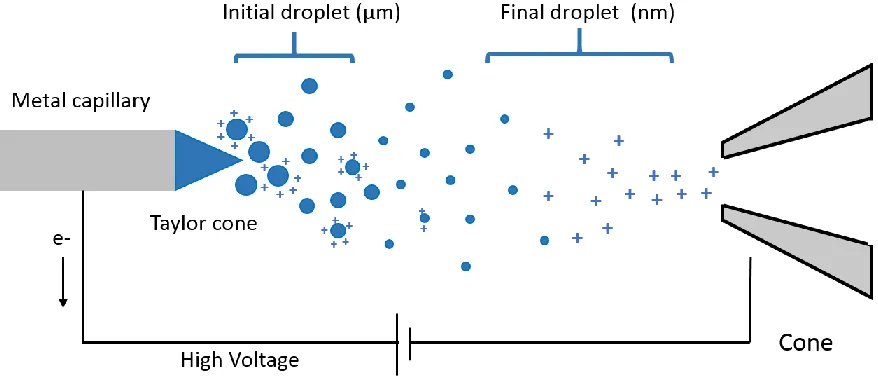
The principle of ESI (Figure 1-1) is to dissolve protein samples in solution which is injected

into a narrow (~100 µm) metal capillary. Upon application of a high voltage (2-3 kV), positive

and negative electrolyte ions will move under the influence of the electric field. Electrons in

solution move away from the capillary tip. Charge balancing redox reaction takes place

including H2O → 2H+ + 2e- + ½ O2. Then the positively charged solution is distorted into a

Taylor cone.32 If the applied field is sufficiently high, the cone tip becomes unstable so that a fine mist of charged droplets is released from the cone. These initial droplets have radii in the

micrometer range. They are positively charged due to excess ions (H+, NH4+, Na+ and K+), and

they are accelerated by electric potential difference between the capillary and the sampling

cone. During the process of acceleration, solvent evaporates rapidly under the influence of

heating and nebulizer gas. As the droplets shrink, their charge to volume ratio increases until

Coulombic repulsion overcomes surface tension.33 Under this circumstance, the number of charges zR is given by Rayleigh limit:34

z

R

=

8𝜋

𝑒

√𝜀

0

𝛾𝑅

(22)

7 where R is the droplet radius, ε0 is the vacuum permittivity, and γ is the surface tension. Droplet

fission occurs at the Rayleigh limit, producing smaller offspring droplets. After several

(23)

8 Figure 1-1 Schematic Depiction of an ESI Source

(24)

9 The mechanisms by which gaseous ions are formed during ESI is still in dispute. The two most

favored mechanisms are the charged-residue mechanism (CRM)35_{and ion-evaporation}

mechanism (IEM)36. In the IEM, it is believed that the charge density becomes sufficiently high due to the large electric field at the surface of droplet, so that ions which carry most of

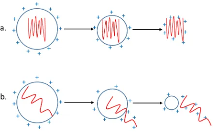
charges are ejected directly out of the nanodroplets.37-40 This model was proved by experiments that explains how metal ions are formed during ESI.41-42 On the other hand, native folded proteins are considered to follow the CRM (Figure 1-2 a.). The idea is that after a succession

of fissions, the droplets would be so small that finally contain only one solute protein. As the

last solvent evaporates from the nanodroplets, the excess charges are retained on proteins so

that droplets become gas-phase ions.35, 43 During the shrinkage, the charges on the molecules are limited by the Rayleigh charge.44 Experimental work in support of the CRM for globular proteins has shown that analyte ions are composed of [M + zRH] zR+, where zR is the Rayleigh

charge of protein-sized water droplets.44-46 Computational studies have also confirmed that globular analytes are trapped deep within the droplet due to the hydration of hydrophilic parts

on proteins, which is not favored to IEM.47-49

However, the CRM is not always suitable for all protein ions. We know that in neutral solution,

most proteins adopt compact folded conformation, which consist of a hydrophobic core and

hydrophilic exterior. Most nonpolar residues are buried in the core, whereas many polar and

charged residues are pointing to the outside.50-51 Once the protein is placed in a denatured environment, they tend to be denatured and hydrophobic interior becomes exposed to the

solvent.52-55 In this case, protein ions are thought to be released via a different type of process, referred to as chain ejection model (CEM) (Figure 1-2 b.).47, 56_{Molecular dynamics}

(25)

10 For unfolded proteins, exposed hydrophobic sites drive the analyte to the droplet surface due

to unfavorable water interaction.57_{In analogy with the IEM, one chain terminus is expelled}

into the gas phase, and then followed by sequential ejection of the remaining chain under the

effect of Coulomb repulsion between positively charged side chains and charges on the droplet.

In conclusion, CRM and CEM apply to the ESI process of folded and unfolded proteins,

(26)

11 Figure 1-2 Mechanisms of Electrospray Ionization.

a. Charged-residue mechanism (CRM): native proteins are retained in the droplets during the shrinkage/fission process. As the last solvent evaporates, excess charges remain on the protein.

(27)

12

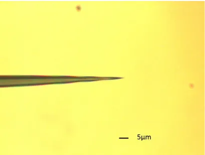
Nanoelectrospray Ionization (Nano ESI)

In terms of ESI techniques, there are two options existing to convert solution phase analytes to

gaseous ions. Regular ESI operates at the flow rate in the µL/min range, using a metal emitter

capillary.30, 58 NanoESI operates with a much smaller spray capillary (Figure 1-3), giving rise to flow rate of less than 100 nL/min.59 NanoESI was first proposed by Wilm, Mann and coworkers.60-61 They pointed out that achieving a low flow rate can be beneficial in many ways. The initial droplets from nanoESI have diameters of less than 200 nm due to the smaller

capillary orifice, which are about 100 to 1000 times smaller than in regular ESI.60 In the aspect of operation, the potential applied on the capillary is around 0.5-1.5 kV, which is significantly

lower than regular ESI, although it always needs an auxiliary pressure to initiate and maintain

a steady flow of solution.62 Considering such low flow rate and small volume of initial droplets, nanoESI can be associated with several advantages. First of all, less sample is required. Only

1-2 µL of sample is loaded directly into the gold-coated glass capillaries.63 Solution is drawn through the capillary without a conventional syringe pump. Secondly, ionization efficiency is

improved, which is supported by a series of experiments.64-67 The ionization efficiency can be characterized as the ratio between the number of detected analyte molecules and the total

number of ions in the solution delivered to the ionization source.68_{It is commonly accepted}

that fission events of the initial droplets lead to lose of a relatively large percentage of charges

and a relatively small percentage of mass.69 Thus, smaller initial droplets produced by nanoESI experience less fission cycles and provide larger fraction of the analyte molecules to become

(28)

13 Figure 1-3 Optical Microscopy Image of a Nanospray Capillary before breaking.

(29)

14 Additionally, nanoESI is believed to have a higher salt tolerance, at least an order of magnitude

better than regular ESI.71-72_{With both techniques, evaporation steadily increases the}

concentration of both analyte and non-volatile salt contaminants in the droplets. NanoESI emits

initial droplets with lower size and higher charge density, which results in a lower number of

fission events. In other words, the Rayleigh charging droplets form earlier without extensive

solvent evaporation. Therefore, the extent of salt enrichment is minimized.62, 71 However, nanoESI also suffers from some drawbacks. It tends to be less robust in terms of signal stability

and reproducibility than regular ESI.73-74

1.2.2 Mass Analyzer

Once the protein ions are produced by ESI and transferred into vacuum, they are ready to be

separated and detected by mass analysis techniques. Mass spectrometer measures mass to

charge ratio, which is given by

m/z

=

[𝑚+𝑧𝐻]

𝑧 (1.3)

assuming that the entire charge is due to excess protons. When the sprayed proteins contain

salt contaminants, the net charge has to take salt ions into account. For example, if Na+ is present in the protein, mass to charge ratio is considered as

m/z

=

[𝑚+(𝑧−𝑖)𝐻+𝑖𝑁𝑎]

𝑧 (1.4)

where 𝑖 refers to the number of sodium ions attached to the protein. Some issues have to be

considered for a high quality mass measurements. First of all is the mass range of the mass

(30)

15 requires a mass analyzer with an extended m/z range. ESI, on the other hand, usually provides

multiply charged ions, so that it would be compatible with many types of mass analyzers.

Another important aspect is the sensitivity. High sensitivity allows mass analyzers to detect

analytes even at low concentration. The third key feature is the resolution. Mass resolution

refers to the minimal difference between two m/z values present in the spectrum that allows a

clear distinction. The classical definition of resolution power R is given by:

R

=

𝑀

𝛥𝑀 (1.5)

where M is the m/z value of a particular ion peak. Historically, according to valley definition,

ΔM is the width of a specified peak at 5% of its height, so that the valley between the two equal

intensity peaks is 10% of the maximum intensity. More recently, another definition is based

on the peak width, where ΔM is the full width at half maximum (FWHM) for each respective

peak.

Quadrupoles

Quadrupoles represent one of the most common devices used in MS. They can be used for ion

storage in which gaseous ions can be confined for a period of time.75 It can also function as ion guide or mass filter. Single quadrupoles were introduced as mass filter for studying proteins.

76-78_{However, the limitation lies in the narrow}_m/z_{range, which is limited to 4000. MS/MS}

experiments can be carried out if three quadrupoles are arranged in series, the so-called triple

quadrupoles.79-80 The first quadrupole is set for selecting precursor ions, while the second one is used as a collision cell that gives rise to collision induced dissociation. The third quadrupole

(31)

16 A quadrupole (Figure 1-4) is composed of two pairs of charged parallel cylindrical metal rods,

one pair positively and the other negatively charged. These four rods are connected diagonally,

so that the same charges are facing each other. Upon the application of a radio frequency (RF)

voltage, ions can pass through because of the potential gradient between the inlet and outlet of

the quadrupoles. A direct current voltage (DC) can be superimposed onto the RF voltage to

implement mass filter operation. The DC voltage provides a stable trajectory for only one m/z

value, while a slightly increase or decrease of m/z value will result in an unstable trajectory so

that they will collide with the rods and never reach the detector. If DC voltage is tuned to zero

which is regarded as an “RF only” mode, the quadrupoles act as an ion guide instead of an ion

filter. It allows all the ions traverse through but confines them in the center, avoiding radial

(32)

17 Figure 1-4 Schematic Description of Quadrupole Operation.

(33)

18

Time-of-Flight (TOF) Mass Analyzer

The time-of-flight concept was introduced half a century ago.82_{It is used more commonly than}

the quadrupole as a mass analyzer due to its wider mass range. The principle of TOF operation

is based on the conversion of potential energy to kinetic energy. The ions are accelerated into

a field free flight tube. In the pusher region, the potential energy Ep is converted to kinetic

energy Ek,

E

p

= E

k

zeU =

1

2

mv

2_(1.6)

where U refers to the acceleration voltage, m refers to the mass of the ion, and v is the velocity

of the ion. The time (t) that ions spend to reach the detector can be described as:

zeU =

1

2

m

(

𝑑 𝑡

)

2

t

=

𝑑 √2𝑒𝑈

√

𝑚

𝑧 (1.7)

where d is the length of the flight tube. 𝑑

√2𝑒𝑈 is independent of the analyte, such that t only

depends on m/z. The ionic signal intensity in the mass spectrum is a function of the arrival time.

However, the simple approach described above gives poor mass resolution due to significant

spread of ions. To improve the performance of the mass analyzer, orthogonal acceleration has

been applied.83-84_{This orthogonal version can reduce the initial velocity distribution along the}

TOF axis, so that ions are focused in an ion beam. Another “correction” for the initial energy

(34)

19 ions that have identical mass and charge first enter the TOF tube, they are accelerated

perpendicularly. However, slight deviations in velocity cause the ions to arrive at the detector

at different times, which decreases the resolution. Upon the setting of reflectron, the faster ion

will penetrate deeper into the decelerating region so that it takes longer to be reflected towards

the detector. The slower ion reaches the reflectron later but its trajectory path is shorter. In this

way, the velocity deviation can be corrected and two ions with the same m/z will reach the

detector at the same time.

Other Mass Analyzers

There are also other types of mass analyzers, such as Fourier Transform Ion Cyclotron

Resonance (FT-ICR) MS and Orbitrap MS, which employ different mechanisms from that in

TOF.86-89 FT-ICR MS is using a magnetic field to force ions into a cyclotron motion. The measurement of m/z is based on the cyclotron frequency. In Orbitrap MS, ions are placed in an

electrostatic field. Under the influence of a central cylindrical electrode, ions orbit with an

(35)

20 Figure 1-5 Schematic layout of mass spectrometer (Synapt G1) used in this work.

(36)

21

1.3 Ion Mobility Spectrometry (IMS)

The advent of mass spectrometry provides an exciting opportunity to study gaseous protein

ions. However, X-ray crystallography, NMR spectroscopy, and cryo-EM are only applicable

in the condensed phase. Assisting MS for resolving images of solvent-free biomolecules, many

spectroscopic tools are used, in addition to gas phase H/D exchange,91-94_{and computer}

simulations.95-97 Ion mobility spectrometry (IMS) has been combined with mass spectrometry (IMS-MS) to investigate the conformational properties of biomolecules in the gas phase.98-101

Clemmer, and Jarrold were the first to resolve different protein ion structures by IMS.102

Bower’s and Russell’s groups developed early MALDI source with IMS.103 More recently,

Clemmer’s group resolved ESI source with IMS.104

1.3.1 Drift Tube Ion Mobility Spectrometry (DTIMS)

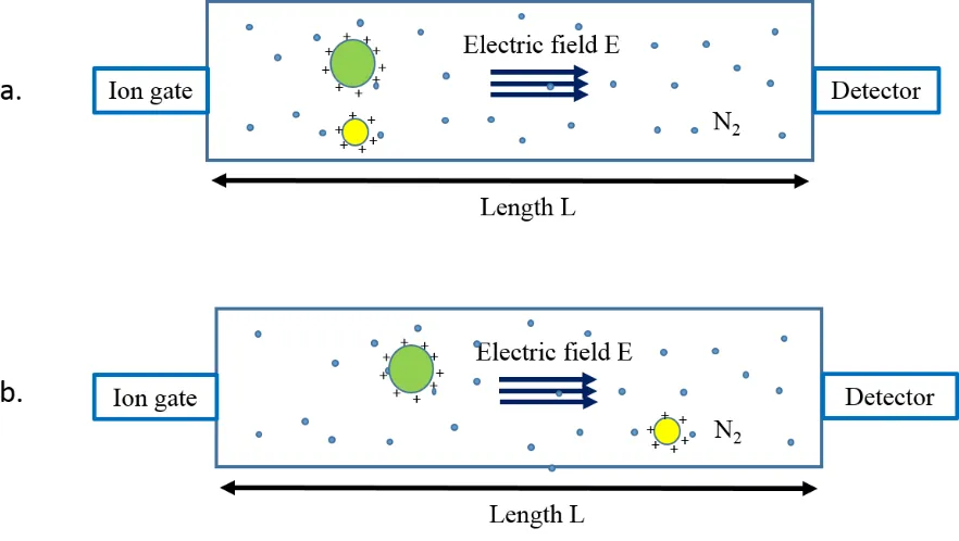
Originally, IMS used simple drift tubes as the separators. A drift tube has a static uniform

electric field along the radial axis to direct ions towards the mass analyzer.105 The drift cell is filled with inert gas, typically helium. A packet of ions is released by an ion gate. Under the

influence of the weak electric field, injected ions traverse the drift region with a velocity

v

d

= K × E

(1.8)

v

d

=

𝐿

𝑡_𝑑

E

=

𝑉

𝐿

where E corresponds to the electric field, and V is the voltage applied across the drift cell. K

(37)

22 hence K contains terms of ion charge state, shape and gas pressure. Individual components

within analyte packet can be separated because of differences in mobility. Drift time (td), based

on the common concept, is determined by the velocity and the length of drift tube (L). On the

other hand, considering the differences among laboratories, K is usually normalized to standard

conditions, yielding the reduced mobility (K0):

K

0

=

𝐿

2

𝑡𝑑 𝑉

×

273.2 𝐾 𝑇

×

𝑃

760 𝑇𝑜𝑟𝑟 (1.9)

where P and T correspond to the pressure and temperature of buffer gas, respectively.106_The

collision cross section (Ω) can be related to the drift time according to Mason-Schamp

equation:100, 106-108

Ω = (

18𝜋

µ𝑘_𝑩𝑇

)

1/2 𝑒𝐸 16𝑁𝐿

𝑇 273.2 𝐾

760 𝑇𝑜𝑟𝑟

𝑃

𝑡

𝑑

𝑧

(1.10)

where z corresponds to the ion charge; kB is the Boltzmann's constant; N is the number density

of the buffer gas; and µ refers to the reduced mass of ion and buffer gas. From this relationship,

we can conclude that for the ions with same charges, large species experience a stronger

resistance than small ions because of collisions with gas molecules. Hence, the drift time (td)

is longer for large ions (Figure 1-6). On the other hand, ions with more charges experience a

larger force during the moving process. Therefore, they traverse more quickly. In consequence,

in IMS, drift time is dependent on collision cross section, as well as ion charge state (td ~ Ω/z).

In comparison, MS separates ions according to m/z. IMS and MS, therefore, are

(38)

23 Figure 1-6 Drift Time IMS Separator (DTIMS).

(39)

24 The CCSs determined from DTIMS provides information for ion shapes. It can be compared

with data derived from X-ray crystallography and NMR spectrometry. DTIMS is superior of

its high resolving power that R can reach 100 Ω/ΔΩ.109 However, it suffers from poor sensitivity due to the low duty cycle and due to ion radial diffusion beyond the extreme

diameter of sampling apertures.110 Duty cycle is related to the percentage of ions detected relative to those enter into the drift cell. This drawback can be effectively overcome by

applying an ion trap before injecting ions into the drift tube, which can accumulate ions while

a previous pulse is being separated.111-112 Another solution to improve duty cycle is to use MALDI as the ionization source, which can provide pulsed ion plume for mobility

separation.113-114 Ion radial diffusion can be lowered by use of a periodic focussing DC drift tube.115

1.3.2 Drift Field and Resolution

The behavior of an ion drifting through buffer gas is dependent on the ratio of electric field

strength to buffer gas number density, E/N.99, 106. At low E/N, the velocity of ions is small compared to the thermal velocity of buffer gas. In this case, the mobility is independent on the

field strength and cross-section measurement report on correspond to the average of all ion

orientations. Under high-field conditions, the mobility may increase or decrease, such that this

regime is usually avoided.116-118

The IMS resolution is given by R = t/Δt. According to Revercomb and Mason119, it can be approximated as:

𝑡 𝛥𝑡

≈

(

𝐿𝐸𝑧𝑒 16𝑘_𝐵𝑇𝑙𝑛2

)

1

(40)

25 where Δt corresponds to the full width at half-maximum of a peak, kB refers to Boltzmann’s

constant, L is the length of the drift tube, and E is the electric field applied along the drift region.

This shows that increasing the drift field or length, or decreasing the temperature is helpful to

improve the resolution.

1.3.3 Collision Cross Section (CCS)

The idea of IMS is that ion packages are exposed to an electric field in the presence of a

background gas. IMS separates gaseous ions according to Ω/z, where Ω and z are the collision

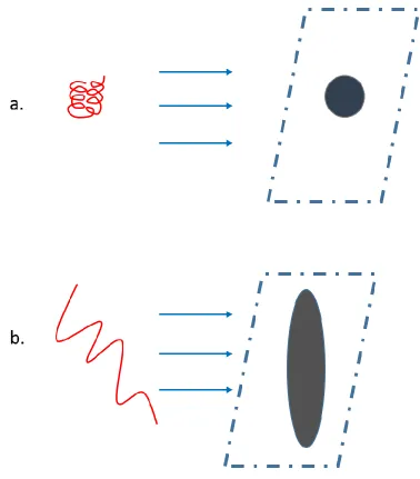
cross section and the charge state, respectively. To a first approximation, collision cross section

represents a rotationally averaged projection area involved in ion-buffer gas collisions.120 CCS can represent protein “size”. For example, unfolded proteins will have larger Ω values than

tightly folded species (Figure 1-7). In order to calculate the collision cross section, Shvartsburg

and Jarrold developed a program called MOBCAL to determine theoretical CCS values based

on input coordinate files, derived from X-ray crystallography, NMR studies, or MD

simulations.121-123 Three models are commonly used in MOBCAL: Projection approximation (PA),124 exact hard sphere scattering method (EHSS),125 and trajectory method (TM).122 The simplest approach is the PA. The CCS is determined by averaging all possible orientations

when the particle rotates. However, this method ignores the long-distance interactions and the

scattering process between the ion and buffer gas. As an improvement, the EHSS method

calculates CCSs by averaging the momentum transfer cross section. It takes into account

(41)

26 scattering events, long-range interactions and multiple collisions. The only weakness we have

(42)

27 Figure 1-7 An Approximate Schematic Diagram of Collision Cross Section (CCS).

(43)

28

1.3.4 Travelling Wave Ion Mobility Spectrometry (TWIMS)

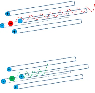
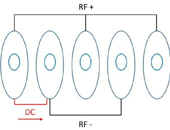
A different approach to mobility separate ions is using travelling wave voltages. This

preference is caused by the availability of commercial TWIMS instrument in the recent

years.110 A TWIMS device comprises a series of ring electrodes that form a stacked ring ion guides.127 The ion guides are arranged orthogonally to the ion transmission direction. Opposite phases of a radio frequency (RF) voltage are applied to adjacent electrodes to provide radial

potential barrier (Figure 1-8).128 The ions are trapped in these potential wells so that ion diffusion can be minimized during transmission process. If the ion traps are sufficiently deep,

some ions can be prevented and never exit from the cell.129 In order to propel ions, a direct current (DC) voltage is superimposed on the RF voltage to a pair of ring electrodes. This DC

voltage is transient on one pair of rings and then switches to next pair downstream at regular

time. Therefore, the potential hills are generated continuously and provide propagating pulse

that push the ions forward (travelling wave ion guide - TWIG). There is nitrogen gas filled in

(44)

29 Figure 1-8 Travelling Wave Ion Guide (TWIG).

(45)

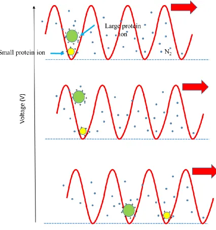
30 Ion mobility separation is achieved by the effect of travelling wave voltage and collisions with

buffer gas (Figure 1-9). During the drifting process, all the ions are propelled in the direction

that the wave is travelling. Ion species of high mobility are more likely to keep up with the

waves. While the ions that have low mobility are impeded by collisions and slip behind the

waves. Therefore, different structural ions would exit at different time and mobility-based

separation takes place. It has been found empirically130 that tdin TWIMS is described as

Ω =

z × F ×

𝑡

_𝑑𝐵 (1.12)

where F and B are constant that have to be determined experimentally. Hence, TWIMS data

have to be calibrated based on drift tube reference values.105, 107, 131-132

For the Synapt instrument used in this work (Figure 1-5), there are three TWIGs. The trap ion

guide is used to accumulate ions and then release them into the IM ion guide. The IM ion guide

is the ion mobility separator. It is gas tight except the entrance and exit apertures. The transfer

(46)

31 Figure 1-9 Travelling Wave IMS Separator.

(47)

32 The characteristics of mobility separation of TWIMS is very similar to those of DTIMS. The

advantage of TWIMS includes high transmission efficiency due to the ion accumulation and

radial ion confinement.110 The transit time of ions through the collision cell is reduced which makes it more compatible for combining with a tandem mass spectrometer where fast mass

scanning or switching is required. For example, application of TWIMS increased the rate at

which biological samples could be screened, which enables the efficient detection and

identification of impurities in therapeutic drugs.133_{The sensitivity is also not compromised}

when acquiring mobility mode.127 However, the resolution of TWIMS is not as high as in DTIMS. Recently, there have been improvements to increase the resolution by raising TWIMS

operating pressure, using a helium entry cell, and increasing field and amplitude of the

T-wave.134 All these factors helped enhancing resolution to 45 (Ω / ΔΩ), which is four times that of the original version.

1.4 Scope of this Thesis

In this work, we employ TWIMS combined with mass spectrometry to investigate the

conformational properties of electrosprayed protein ions in the gas phase. The drift time data

obtained from experiments have to be calibrated based on reference CCS values. The calibrated

CCSs can be compared with the values calculated from model structures obtained by X-ray

crystallography and NMR spectroscopy and molecular dynamics (MD) simulations

In chapter 2, we revisit the calibration issue related to collisional activation. Exciting protocol

was found to be quite convoluted and do not address a key problem, i.e, the fact that Ω value

can be strongly dependent on experimental conditions. We propose a simplified calibration

(48)

33 In chapter 3, the question whether electrosprayed protein ions retain solution-like

conformations remains is addressed. We employ TWIMS to compare the gas-phase CCSs with

the values calculated from other techniques which provide condensed phase structures. We

also use MD simulations to provide computational structures as another reference. In addition,

we use two types of electrospray ionization sources to perform the IMS experiments on four

different proteins. Thus, comparisons between the two sources can be made in terms of

(49)

34

1.5 References

1. Wu, Y.; Engen, J. R., Analyst 2004, 129 (4), 290-296.

2. Pauling, L.; Corey, D. R.; Branson, H. R., Proc. Natl. Acad. Sci. U.S.A. 1951, 37,

205-210.

3. Pauling, L.; Corey, R. B., Proc Natl Acad Sci USA 1951, 37 (5), 251-256.

4. Southall, N. T.; Dill, K. A.; Haymett, A. D. J., J. Phys. Chem. B 2002, 106, 521-533.

5. Widom, B.; Bhimalapuram, P.; Koga, K., Phys. Chem. Chem. Phys. 2003, 5,

3085-3093.

6. Anfinsen, C. B., Science 1973, 181, 223-230.

7. Miranker, A.; Robinson, C. V.; Radford, S. E.; Dobson, C. M., FASEB J. 1996, 10,

93-101.

8. Bai, Y.; Sosnick, T. R.; Leland, M.; Englander, S. W., Science 1995, 269 (5221),

192-197.

9. Currin, A.; Swainston, N.; Day, P. J.; Kell, D. B., Chem. Soc. Rev. 2015, 44 (5),

1172-1239.

10. Ingle, D. J.; Crouch, S. R., Spectrochemical Analysis. Prentice Hall, New Jersey, 1988.

11. Nienhaus, K.; Nienhaus, G. U., Probing Heme Protein-Ligand Interactions by

UV/Visible Absorption Spectroscopy. In Protein-Ligand Interactions, Ulrich Nienhaus, G.,

(50)

35 12. Engler, N.; Ostermann, A.; Gassmann, A.; Lamb, D. C.; Prusakov, V. E.; Schott, J.;

Schweitzer-Stenner, R.; Parak, F. G., Biophys. J. 2000, 78 (4), 2081-2092.

13. Kelly, S. M.; Price, N. C., Curr Protein Pept Sci. 2000, 1 (4), 349-384.

14. Chen, Y.; Barkley, M. D., Biochemistry 1998, 37, 9976-9982.

15. Rhodes, G., Crystallography Made Crystal Clear. 2nd ed.; Academic Press: San Diego,

2000; p pp 29-37.

16. Read, R. J., Structure 1996, 4 (1), 11-14.

17. Moffat, K., Chem.Rev. 2001, 101, 1569-1581.

18. Petsko, G. A.; Ringe, D., Curr. Op. Chem. Biol. 2000, 4 (1), 89-94.

19. Woodward, C., Trends Biochem. Sci. 1993, 18, 359-360.

20. Li, R.; Woodward, C., Protein Sci. 1999, 8 (8), 1571-1590.

21. Cala, O.; Guilliere, F.; Krimm, I., Anal. Bioanal. Chem. 2014, 406 (4), 943-956.

22. Unger, V. M., Curr. Op. Struct. Biol. 2001, 11 (5), 548-554.

23. Urnavicius, L.; Zhang, K.; Diamant, A. G.; Motz, C.; Schlager, M. A.; Yu, M. M.; Patel,

N. A.; Robinson, C. V.; Carter, A. P., Science 2015, 347 (6229), 1441-1446.

24. Griffiths, I. W., Rapid communications in mass spectrometry : RCM 1997, 11 (1),

3-16.

(51)

36 26. Tanaka, K.; Waki, H.; Ido, Y.; Akita, S.; Yoshida, Y.; Yoshida, T.; Matsuo, T., Rapid

communications in mass spectrometry : RCM 1988, 2 (8), 151-153.

27. Markides, K.; Gräslund, A., The Royal Swedish Academy of Sciences 2002, 1-13.

28. Chang, W. C.; Huang, L. C.; Wang, Y. S.; Peng, W. P.; Chang, H. C.; Hsu, N. Y.; Yang,

W. B.; Chen, C. H., Anal. Chim. Acta 2007, 582, 1-9.

29. Keller, B. O.; Li, L., J. Am. Soc. Mass Spectrom. 2001, 12, 1055-1063.

30. Fenn, J. B., Angew. Chem. Int. Ed. 2003, 42, 3871-3894.

31. El-Aneed, A.; Cohen, A.; Banoub, J., Appl. Spectrosc. Rev. 2009, 44 (3), 210-230.

32. Taylor, G.; Mcewan, A. D., J. Fluid Mech 1965, 22, 1-15.

33. Iavarone, A. T.; Williams, E. R., J. Am. Chem. Soc. 2003, 125, 2319-2327.

34. Rayleigh, L., phil. Mag. 1882, 14 (87), 184-186.

35. Dole, M.; Mack, L. L.; Hines, R. L.; Mobley, R. C.; Ferguson, L. D.; Alice, M. B., J.

Chem. Phys. 1968, 49, 2240-2249.

36. Iribarne, J. V.; Thomson, B. A., J. Chem. Phys. 1976, 64, 2287-2294.

37. Nguyen, S.; Fenn, J. B., Proc. Natl. Acad. Sci. U.S.A. 2007, 104, 1111-1117.

38. Zhan, D.; Rosell, J.; Fenn, J. B., J. Am. Soc. Mass Spectrom. 1998, 9, 1241-1247.

39. Fenn, J. B., J. Am. Soc. Mass Spectrom. 1993, 4, 524-535.

40. Gamero-Castaño, M.; de la Mora, F. J., Anal. Chim. Acta 2000, 406, 67-91.

(52)

37 42. Gamero-Castaño, M.; de la Mora, F., J. Mass Spectrom. 2000, 35, 790-803.

43. Hogan, C. J.; Carroll, J. A.; Rohrs, H. W.; Biswas, P.; Gross, M. L., Anal. Chem. 2009,

81, 369-377.

44. Labowsky, M.; Fenn, J. B.; Fernandez de la Mora, J., Anal. Chim. Acta 2000, 406,

105-118.

45. Kebarle, P.; Verkerk, U. H., Mass Spec. Rev. 2009, 28 (6), 898-917.

46. Heck, A. J. R.; Van den Heuvel, R. H. H., Mass Spectrom. Rev. 2004, 23, 368-389.

47. Ahadi, E.; Konermann, L., J. Phys. Chem. B 2012, 116, 104-112.

48. Patriksson, A.; Marklund, E.; van der Spoel, D., Biochem 2007, 46, 933-945.

49. Steinberg, M. Z.; Breuker, K.; Elber, R.; Gerber, R. B., Phys. Chem. Chem. Phys. 2007,

9, 4690-4697.

50. Fersht, A. R., Structure and Mechanism in Protein Science. W. H. Freeman & Co.:

New York, 1999.

51. Rose, G. D.; Geselowitz, A. R.; Lesser, G. J.; Lee, R. H.; Zehfus, M. H., Science 1985,

229 (4716), 834-838.

52. Kuprowski, M. C.; Konermann, L., Anal. Chem. 2007, 79, 2499-2506.

53. Dobo, A.; Kaltashov, I. A., Anal. Chem. 2001, 73, 4763-4773.

54. Konermann, L.; Douglas, D. J., J. Am. Soc. Mass Spectrom. 1998, 9, 1248-1254.

(53)

38 56. Konermann, L.; Rodriguez, A. D.; Liu, J., Anal. Chem. 2012, 84, 6798–6804.

57. Konermann, L.; Ahadi, E.; Rodriguez, A. D.; Vahidi, S., Anal. Chem. 2013, 85, 2-9.

58. Covey, T. R.; Thomson, B. A.; Schneider, B. B., Mass Spectrom. Rev. 2009, 28,

870-897.

59. Wang, W.; Kitova, E. N.; Klassen, J. S., Anal. Chem. 2003, 75, 4945-4955.

60. Wilm, M.; Mann, M., Anal. Chem. 1996, 68, 1-8.

61. Wilm, M.; Shevchenko, A.; Houthaeve, T.; Breit, S.; Schweigerer, L.; Fotsis, T.; Mann,

M., Nature 1996, 379, 466-469.

62. Benesch, J. L. P.; Ruotolo, B. T.; Simmons, D. A.; Robinson, C. V., Chem. Rev. 2007,

107, 3544-3567.

63. Yuill, E. M.; Sa, N. Y.; Ray, S. J.; Hieftje, G. M.; Baker, L. A., Anal. Chem. 2013, 85

(18), 8498-8502.

64. Oosterkamp, A. J.; Gelpi, E.; Abian, J., J. Mass Spectrom. 1998, 33 (10), 976-983.

65. Chang, Y. Z.; Chen, Y. R.; Her, G. R., Anal. Chem. 2001, 73 (21), 5083-5087.

66. Bendahl, L.; Hansen, S. H.; Olsen, J., Rapid Commun. Mass Spectrom. 2002, 16 (24),

2333-2340.

67. Jecklin, M. C.; Touboul, D.; Bovet, C.; Wortmann, A.; Zenobi, R., J. Am. Soc. Mass

Spectrom. 2008, 19, 332-343.

68. Marginean, I.; Page, J. S.; Tolmachev, A. V.; Tang, K. Q.; Smith, R. D., Anal. Chem.

(54)

39 69. Grimm, R. L.; Beauchamp, J. L., Anal. Chem. 2002, 74 (24), 6291-6297.

70. Geromanos, S.; Freckleton, G.; Tempst, P., Anal. Chem. 2000, 72 (4), 777-790.

71. Juraschek, R.; Dulcks, T.; Karas, M., J. Am. Soc. Mass Spectrom. 1999, 10, 300-308.

72. Karas, M.; Bahr, U.; Dulcks, T., Front Sci. Ser. 2000, 366 (6-7), 669-676.

73. Gabelica, V.; Vreuls, C.; Filee, P.; Duval, V.; Joris, B.; De Pauw, E., Rapid Commun.

Mass Spectrom. 2002, 16, 1723-1728.

74. Bovet, C.; Wortmann, A.; Eiler, S.; Granger, F.; Ruff, M.; Gerrits, B.; Moras, D.;

Zenobi, R., Protein Sci. 2007, 16 (5), 938-946.

75. March, R. E., J. Mass Spectrom. 1997, 32 (4), 351-369.

76. Iribarne, J. V.; Dziedzic, P. J.; Thomson, B. A., Int. J. Mass. Spectrom. 1983, 50,

331-347.

77. Smith, R. D.; Loo, J. A.; Baringa, C. J.; Edmonds, C. G.; Udseth, H. R., J. Am. Soc.

Mass Spectrom. 1990, 1, 53-65.

78. Mirza, U. A.; Cohen, S. L.; Chait, B. T., Anal. Chem. 1993, 65, 1-6.

79. Cox, K. A.; Julian, R. K.; Cooks, R. G.; Kaiser, R. E., J. Am. Soc. Mass Spectrom. 1994,

5, 127-136.

80. Chernushevich, I. V.; Loboda, A. V.; Thomson, B. A., J. Mass Spectrom. 2001, 36 (8),

849-865.

81. Steel, C.; Henchman, M., J. Chem. Ed. 1998, 75 (8), 1049-1054.

(55)

40 83. Cotter, R. J., Anal. Chem. 1999, 71 (13), 445A-451A.

84. Verentchikov, A. N.; Ens, W.; Standing, K. G., Anal. Chem. 1994, 66 (1), 126-133.

85. Mamyrin, B. A., Int. J. Mass Spectrom. 2001, 206 (3), 251-266.

86. Comisaro.Mb; Marshall, A. G., Chem. Phys. Lett. 1974, 25 (2), 282-283.

87. Marshall, A. G., Int. J. Mass Spectrom. 2000, 200 (1-3), 331-356.

88. Makarov, A., Anal. Chem. 2000, 72, 1156-1162.

89. Hardman, M.; Makarov, A., Anal. Chem. 2003, 75, 1699-1705.

90. Hu, Q.; Noll, R. J.; Li, H.; Makarov, A.; Hardman, M.; Cooks, R. G., J. Mass Spectrom.

2005, 40, 430-443.

91. Goswami, D.; Tuske, S.; Pascal, B. D.; Bauman, J. D.; Patel, D.; Arnold, E.; Griffin, P.

R., Anal.Chem 2015, 87 (7), 4015-4022.

92. Keppel, T. R.; Weis, D. D., J. Am. Soc. Mass Spectrom. 2015, 26 (4), 547-554.

93. Zhang, Z. Q.; Smith, D. L., Protein Sci. 1993, 2 (4), 522-531.

94. Khakinejad, M.; Kondalaji, S. G.; Maleki, H.; Arndt, J. R.; Donohoe, G. C.; Valentine,

S. J., J. Am. Soc. Mass Spectrom. 2014, 25 (12), 2103-2115.

95. Cornell, W. D.; Cieplak, P.; Bayly, C. I.; Gould, I. R.; Merz, K. M.; Ferguson, D. M.;

Spellmeyer, D. C.; Fox, T.; Caldwell, J. W.; Kollman, P. A., J. Am. Chem. Soc. 1995, 117 (19),

5179-5197.

96. Steinberg, M. Z.; Elber, R.; McLafferty, F. W.; Gerber, R. B.; Breuker, K.,

(56)

41 97. Saikusa, K.; Fuchigami, S.; Takahashi, K.; Asano, Y.; Nagadoi, A.; Tachiwana, H.;

Kurumizaka, H.; Ikeguchi, M.; Nishimura, Y.; Akashi, S., Anal. Chem. 2013, 85 (8),

4165-4171.

98. Wyttenbach, T.; von Helden, G.; Bowers, M. T., J. Am. Chem. Soc. 1996, 118,

8355-8364.

99. Clemmer, D. E.; Jarrold, M. F., J. Mass Spectrom. 1997, 32, 577-592.

100. Konijnenberg, A.; Butterer, A.; Sobott, F., BBA-Proteins Proteomics 2013, 1834 (6),

1239-1256.

101. Lee, J. W.; Kim, H. I., Analyst 2015, 140 (2), 661-669.

102. Clemmer, D. E.; Hudgins, R. R.; Jarrold, M. F., J. Am. Chem. Soc. 1995, 117,

10141-10142.

103. Gillig, K. J.; Ruotolo, B.; Stone, E. G.; Russell, D. H.; Fuhrer, K.; Gonin, M.; Schultz,

A. J., Anal. Chem. 2000, 72 (17), 3965-3971.

104. Myung, S.; Wiseman, J. M.; Valentine, S. J.; Takats, Z.; Cooks, R. G.; Clemmer, D. E.,

J. Phys. Chem. B 2006, 110 (10), 5045-5051.

105. Bush, M. F.; Hall, Z.; Giles, K.; Hoyes, J.; Robinson, C. V.; Ruotolo, B. T., Anal. Chem.

2010, 82, 9667-9565.

106. Mason, E. A.; McDaniel, E. W., Wiley 1988.

107. Ruotolo, B. T.; Benesch, J. L. P.; Sandercock, A. M.; Hyung, S.-J.; Robinson, C. V.,

Nat. Protocols 2008, 3, 1139-1152.

108. Kanu, A. B.; Dwivedi, P.; Tam, M.; Matz, L. M.; Hill, H. H., J. Mass Spectrom. 2008,

(57)

42 109. Lanucara, F.; Holman, S. W.; Gray, C. J.; Eyers, C. E., Nature Chemistry 2014, 6 (4),

281-294.

110. Pringle, S. D.; Giles, K.; Wildgoose, J. L.; Williams, J. P.; Slade, S. E.; Thalassinos,

K.; Bateman, R. H.; Bowers, M. T.; Scrivens, J. H., Int. J. Mass Spectrom. 2007, 261, 1-12.

111. Hoaglund, C. S.; Valentine, S. J.; Clemmer, D. E., Anal. Chem. 1997, 69 (20),

4156-4161.

112. Wyttenbach, T.; Kemper, P. R.; Bowers, M. T., Int. J. Mass Spectrom. 2001, 212

(1-3), 13-23.

113. Gillig, K. J.; Ruotolo, B. T.; Stone, E. G.; Russell, D. H., Int. J. Mass Spectrom. 2004,

239 (1), 43-49.

114. Woods, A. S.; Ugarov, M.; Egan, T.; Koomen, J.; Gillig, K. J.; Fuhrer, K.; Gonin, M.;

Schultz, J. A., Anal. Chem. 2004, 76 (8), 2187-2195.

115. McLean, J. A.; Ruotolo, B. T.; Gillig, K. J.; Russell, D. H., Int. J. Mass Spectrom. 2005,

240 (3), 301-315.

116. Buryakov, I. A.; Krylov, E. V.; Nazarov, E. G.; Rasulev, U. K., Int. J. Mass Spectrom.

Ion Proc. 1993, 128 (3), 143-148.

117. Purves, R. W.; Guevremont, R.; Day, S.; Pipich, C. W.; Matyjaszczyk, M. S., Rev. Sci.

Inst. 1998, 69 (12), 4094-4105.

118. Shvartsburg, A. A.; Mashkevich, S. V.; Smith, R. D., J. Phys. Chem. A 2006, 110 (8),

2663-2673.

119. Revercomb, H. E.; Mason, E. A., Anal. Chem. 1975, 47 (7), 970-983.

(58)

43 121. Shvartsburg, A. A.; Jarrold, M. F., Chem. Phys. Lett. 1996, 261 (1–2), 86-91.

122. Shvartsburg, A. A.; Schatz, G. C.; Jarrold, M. F., J. Chem. Phys. 1998, 108 (6),

2416-2423.

123. Mesleh, M. F.; Hunter, J. M.; Shvartsburg, A. A.; Schatz, G. C.; Jarrold, M. F., J. Phys.

Chem. 1996, 100 (40), 16082-16086.

124. Wyttenbach, T.; vonHelden, G.; Batka, J. J.; Carlat, D.; Bowers, M. T., J. Am. Soc.

Mass Spectrom. 1997, 8 (3), 275-282.

125. Shvartsburg, A. A.; Smith, R. D., J. Am. Soc. Mass Spectrom. 2008, 19 (9), 1286-1295.

126. Zubarev, R. A.; Horn, D. M.; Fridriksson, E. K.; Kelleher, N. L.; Kruger, N. A.; Lewis,

M. A.; Carpenter, B. K.; McLafferty, F. W., Anal. Chem. 2000, 72 (3), 563-573.

127. Giles, K.; Pringle, S. D.; Worthington, K. R.; Little, D.; Wildgoose, J. L.; Bateman, R.

H., Rapid communications in mass spectrometry : RCM 2004, 18 (20), 2401-14.

128. Tolmachev, A. V.; Kim, T.; Udseth, H. R.; Smith, R. D.; Bailey, T. H.; Futrell, J. H.,

Int. J. Mass Spectrom. 2000, 203 (1-3), 31-47.

129. Lynn, E. C.; Chung, M. C.; Han, C. C., Rapid communications in mass spectrometry :

RCM 2000, 14 (22), 2129-2134.

130. Wildgoose, J.; Giles, K.; Pringle, S. D.; Koeniger, S. L.; Valentine, J. S.; Bateman, R.

H.; Clemmer, D. E., A comparison of travelling wave and drift tube ion mobility separations.

In Proc. 54th ASMS Conference on Mass Spectrometry & Allied Topics, Seattle, WA.

131. Shvartsburg, A. A.; Smith, R. D., Anal. Chem. 2008, 80, 9689–9699.

(59)

44 133. Esquenazi, E.; Daly, M.; Bahrainwala, T.; Gerwick, W. H.; Dorrestein, P. C., Bioorg.

Med. Chem. 2011, 19 (22), 6639-6644.

134. Giles, K.; Williams, J. P.; Campuzano, I., Rapid Commun. Mass Spectrom. 2011, 25,

(60)

45

Chapter 2 - Calibration Issues in TWIMS

2.1 Introduction

IMS separates gaseous ions according to Ω/z, where Ω and z are the collision cross section and

the charge state, respectively. To a first approximation, Ω represents a rotationally averaged

projection area.1 Ion packages are exposed to an electric field in the presence of a background gas. In drift tube IMS the electric field E is static, and the ions traverse a drift region of length

L. Ω can then be determined using the relationships2-4

Ω

= z × C × t

d (2.1a)

C

=

𝑒𝐸 16𝑁𝐿

(

18𝜋 µ𝑘_𝐵𝑇

)

1/2760 𝑇𝑜𝑟𝑟 𝑝

𝑇

273.2 𝐾 (2.1b)

with the reduced mass µ, elementary charge e, gas number density N, temperature T,

Boltzmann’s constant kB, and gas pressure p.

Recent years have witnessed the rapid growth of traveling wave (TW) IMS, where ions “surf”

on DC waves within a stacked-ring RF ion guide.4-7 The primary difference from DTIMS is that the electric field is not constant and uniform. The transit time decreases with mobility due

to the pulsed voltage. It has been found empirically8 that tdin TWIMS is related to Ω via

Ω =

z × F ×

𝑡

_𝑑𝐵 (2.2)

where F and B cannot be calculated from first principles. (eq. 2.1) Instead, TWIMS data have

(61)

46 Extracting quantitative structural information from IMS data is surprisingly difficult. An

experimental Ω value represents a single number that may be consistent with many different

analyte conformations. Several methods have been developed for predicting Ω values of model

structures, but these methods yield results that can differ by 30% or more.1, 14 X-ray data are often assumed to provide plausible gas phase model structures, although crystal packing and

residual water provide an environment that is very different from the vacuum.15 Molecular dynamics (MD) simulations provide insights into the behavior of proteins in the absence of

solvent,16-19 but MD force fields are parametrized for bulk solution.20 Eq. 2.1, which provides the foundation of macromolecular IMS, only represents an approximate solution of a rigorous

kinetic treatment.21 The commonly used approach of calibrating TWIMS Ω values measured in N2 on the basis of published He drift tube data may introduce additional issues.7-8, 18, 22-26

Briefly, the mobility in He is higher than that in N227, at a given pressure, lower T-wave

amplitude has to be used in with He. This can be explained that the separation has a high

mobility limit, so that ion species above this limit would just surf on a single wave without

mobility separation. Only the ions below the limit can be overtaken by the wave and experience

the forward and reverse fields of the pulse.28 However, the lower amplitudes has been proved empirically as a result of lower gas pressure4-5_{, which causes lower resolution. On the other}

hand, in order to achieve a high resolution, increasing N2 pressure can give rise to another

problem that a higher gas flow rate is applied and more energy is required to drive ions, which

results in ion losses through scattering and fragmentation.29

Like other TWIMS calibration strategies,30-32 the procedure used here relies on reference data Ωref measured in He. Calibrated TWIMS Ω values therefore represent “effective” He collision

(62)

47 should correct for systematic differences between mobility in He and in N2. F in eq. 2.2 is

occasionally expressed as F = C × A, where A is an empirical constant and C is defined in eq.

2.1b.9, 34 This notation suggests that F follows a µ-1/2 dependence with µ = mM/(m+M), where

m and M are the gas and analyte masses, respectively. To our knowledge, it has never been

proven that A is independent of µ.8 Therefore, the assumption that F is proportional to µ-1/2

seems unjustified. Existing TWIMS calibration protocols nonetheless advocate a µ-1/2

correction.3, 10_{Luckily, this correction is negligible for proteins, where}_{M >> m}_{such that µ ≈}

m. For example, Hb has µ = 27.99 Da, whereas Ubq has µ = 27.91 Da resulting in Δ(µ-1/2) ≈

0.1%. Similar considerations apply to measured td values which, strictly speaking, should be

corrected for the time that the ions spend outside the drift region. This issue is important for

some instruments,10 but it is insignificant for the TWIMS device considered here. The TWIMS

td correction is on the order of 0.5% and its weak (m/z)1/2 dependence implies that different

analytes are affected to a very similar extent.3 In summary, µ and td corrections are unnecessary

for the type of instrument used here, considering (i) the empirical origin eq. 2.28 and (ii) the small magnitude of these corrections which is within the scatter of the calibration plots.

2.2 Experimental

2.2.1 Sample Preparation

Bovine ubiquitin (Ubq, 8565 Da), horse heart cytochrome c (Cyt, 12359 Da), and equine

holo-myoglobin (hMb, 17568 Da) were purchased from Sigma (St. Louis, MO). The calibrant mix

Using Ion Mobility Spectrometry to Study Protein Conformations in the Gas Phase

Scholarship@Western

Scholarship@Western

Using Ion Mobility Spectrometry to Study Protein Conformations

Using Ion Mobility Spectrometry to Study Protein Conformations

in the Gas Phase

in the Gas Phase

Using Ion Mobility Spectrometry to Study Protein

Conformations in the Gas Phase

(Thesis format: Integrated-Article)

by

Yu Sun

Graduate Program in Chemistry

A thesis submitted in partial fulfillment

of the requirements for the degree of

Master of Science

The School of Graduate and Postdoctoral Studies

The University of Western Ontario

London, Ontario, Canada

Abstract

Keywords:

Statement of Co-Authorship

Acknowledgement

Table of Contents

List of Tables

List of Figures

List of Symbols and Abbreviations

Chapter 1

- Introduction

1.1

Protein Structure and Function

N

→

Δ

G =

Δ

H – T

Δ

S

1.2

Mass Spectrometry

z

=

√𝜀

𝛾𝑅

m/z

=

m/z

=

R

=

E

= E

zeU =

mv

zeU =

m

(

)

t

=

√

1.3

Ion Mobility Spectrometry (IMS)

v

= K × E

v

=

E

=

K

=

×

×

Ω = (

)

𝑡

𝑧

≈

(