Using Machine Learning for Precision Measurements
DimitriBourilkov1,∗
1University of Florida, PO Box 118440, Gainesville, FL 32611, USA
Abstract.The use of machine learning techniques for classification is well es-tablished. They are applied widely to improve the signal-to-noise ratio and the sensitivity of searches for new physics at colliders. In this study I explore the use of machine learning for optimizing the output of high precision experiments by selecting the most sensitive variables to the quantity being measured. The precise determination of the electroweak mixing angle at the Large Hadron Col-lider using linear or deep neural network regressors is developed as a test case.
1 Physics Motivation
The forward-backward asymmetryAFBof lepton pairs at the Large Hadron Collider (LHC)
around the Z peak is sensitive to the electroweak mixing angle. The potential of the LHC for a precise measurement of this angle has been recognized early on [1]. TraditionallyAFBis
measured from the cosϑdistribution of the electron or negative muon member of the lepton pair in the Collins-Soper frame [2]. This entails transformation of the kinematic variables to this frame, producing the distribution, and then typically performing a fit on it to extract the asymmetry, and using it for the electroweak angle measurement. This contribution asks: can we extractAFBdirectly from the experimentally measured quantities, bypassing the standard
procedure, by applying machine learning (ML) techniques? In other words, can we bypass our knowledge of how high energy physics has been done for decades, and replace it by a neural network regressor based on machine learning?
2 Monte Carlo Simulations and Setup
Events are generated using the very popular Monte Carlo generator PYTHIA [3–5] - version 8.210. The parton density functions used are from the CTEQ61 set [6]. The events are generated in the typical acceptance of a generic LHC detector at 13 TeV at different invariant
masses for the final-state lepton (dielectron or dimuon) pair around 70, 91, 200 and 500 GeV. The leptons are required to have pseudorapidity|η| < 2.4 and transverse momentum pT >25GeV. These masses are chosen to follow the change of the asymmetry AFBwith
mass from negative values below the Z peak to positive values above the peak, as exemplified in figure 1 by the measurement of the CMS collaboration at 8 TeV.
Two thousand events are generated at each selected mass. The samples are split in three independent parts:
Figure 1. Example of the observed forward-backward asymmetryAFBat the LHC for|y|<1, as mea-sured by the CMS collaboration at 8 TeV [7].
• 10% for validation
• 15% for testing.
The details of the generation and the number of events for the following studies are sum-marized in table 1. In total slightly below half of the events pass the acceptance cuts and are retained for the analysis. As expected, the acceptance grows for higher masses of the dilepton system.
Table 1.Details of the Monte Carlo simulations with Pythia for different mass bins.
Mass bin Events for Events for All Observed (GeV) Training Val. & Test Events asymmetryAFB
65-75 512 170 682 -0.0643
86.2-96.2 618 206 824 0.0059
195-205 842 280 1122 0.1410
495-505 1022 341 1363 0.2187
Total 2994 997 3991
pseudo-Figure 1. Example of the observed forward-backward asymmetryAFBat the LHC for|y|<1, as mea-sured by the CMS collaboration at 8 TeV [7].
• 10% for validation
• 15% for testing.
The details of the generation and the number of events for the following studies are sum-marized in table 1. In total slightly below half of the events pass the acceptance cuts and are retained for the analysis. As expected, the acceptance grows for higher masses of the dilepton system.
Table 1.Details of the Monte Carlo simulations with Pythia for different mass bins.
Mass bin Events for Events for All Observed (GeV) Training Val. & Test Events asymmetryAFB
65-75 512 170 682 -0.0643
86.2-96.2 618 206 824 0.0059
195-205 842 280 1122 0.1410
495-505 1022 341 1363 0.2187
Total 2994 997 3991
-The following input variables are considered for the ML regressor: dilepton invariant mass m (not used), transverse momentum pT and rapidity y of the dilepton system,
pseudo-rapidityη1or2, transverse momentum pT1or2 and azimuthal angleϕ1or2 for each decay lepton.
The mass is not used because it relates directly to the forward-backward asymmetryAFB, and
the goal is to extract the asymmetry from the decay kinematics and the angles “hidden” inside it, and not from the mass.
The target variable is the observed forward-backward asymmetryAFB. Here a comment
is in order: the asymmetry is traditionally extracted by the angle between the incoming quark initiating the hard interaction of dilepton production (the Drell-Yan process [8]), and the outgoing electron or negative muon. While the charge of the outgoing leptons is measured with high precision at the LHC, there is no information to distinguish which proton provided the quark, and which the anti-quark. In other words, at the LHC the initial state is symmetric. At rapidity y=0 there is no way to measureAFB. When|y|grows, or the dilepton system
gets a “boost”, the probability that the higher momentum initiating parton is a valence quark, and that the lower momentum parton is a sea anti-quark, grows as well. Correspondingly the tagging of quarks and anti-quarks improves when|y|increases away from the center of the
detectors. The bottom line is that events with sizable values of|y|are sensitive toAFB. Still,
this method of tagging has its limits, so the observed values ofAFB, as shown in figure 1,
are typically 2-3 times lower than the real values if perfect knowledge of the initial state was available. In other words, the observed asymmetry is “diluted” compared to the real one, thus reducing the sensitivity to the electroweak mixing angle, and requiring many more events for reaching the target precision.
In this study linear or deep neural network regressors (LR or DNN regressors) are used to extractAFBdirectly from the decay kinematics. The Tensorflow library [9] provides all the
needed functionalities and is applied to “learn” theAFBdirectly from the simulated data.
3 Linear Regressor - Results
For all regressors first a normalization of the input features is applied. All input variables are transformed to span the range [-1, 1]. This linear scaling can help the minimization procedure (e.g. stochastic gradient descent) to perform more smoothly for multi-dimensional problems. The linear regressor encounters difficulties when trying to extract the asymmetry AFB
directly from the input kinematic variables. This is related to the discussion in the previous section. Experimentation shows that the most sensitive variables are the rapidities, and they work better if converted to derived features (also called synthetic features in the Tensorflow documentation), such as the absolute value of the rapidity|y|and of the pseudorapidities|η1|, |η2|. This way they are well tuned and more proportionally connected to the symmetric nature
of the LHC (where the observedAFBis stronger when the dilepton system has higher boost),
●
●
●
●
● ●
●
● ●
●
500
1000
1500
2000
0.09
0.10
0.11
0.12
0.13
0.14
0.15
LR: Root Mean Squared Error vs Epochs
Epochs
RMSE
●
Training
Validation
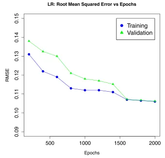
Figure 2. Performance of the linear regressor LR, as measured by the RMSE, as a function of the
epoch.
4 DNN Regressor - Results
The next step is to learn the non-linearities in the dataset and try to achieve better performance compared to the linear regressor results obtained in the previous section. While the LR is a useful first step, the problem is non-linear and a DNN regressor has better chances to enhance the performance, at the price of introducing higher complexity with more parameters to be determined at the learning stage.
The hyperparameters of the deep learning neural network used in this study are: two hidden layers with ten nodes each, ReLu activation, batch size 100, and 2000 epochs. They are selected to match the nature of the problem, neither over-simplifying nor unnecessarily complicating the architecture.
Again normalization of the input features is applied. Various alternatives for the opti-mization algorithms are explored:
• Stochastic Gradient Descent - often used as a starting point
• Adagrad Optimizer - for each model coefficient it modifies adaptively the learning rate
● ● ● ● ● ● ● ● ● ●
500
1000
1500
2000
0.09
0.10
0.11
0.12
0.13
0.14
0.15
LR: Root Mean Squared Error vs Epochs
Epochs
RMSE
●
Training
Validation
Figure 2. Performance of the linear regressor LR, as measured by the RMSE, as a function of the
epoch.
4 DNN Regressor - Results
The next step is to learn the non-linearities in the dataset and try to achieve better performance compared to the linear regressor results obtained in the previous section. While the LR is a useful first step, the problem is non-linear and a DNN regressor has better chances to enhance the performance, at the price of introducing higher complexity with more parameters to be determined at the learning stage.
The hyperparameters of the deep learning neural network used in this study are: two hidden layers with ten nodes each, ReLu activation, batch size 100, and 2000 epochs. They are selected to match the nature of the problem, neither over-simplifying nor unnecessarily complicating the architecture.
Again normalization of the input features is applied. Various alternatives for the opti-mization algorithms are explored:
• Stochastic Gradient Descent - often used as a starting point
• Adagrad Optimizer - for each model coefficient it modifies adaptively the learning rate
and lowers it over the course of the training. This is known to perform well for convex
problems, bur is not necessarily optimal for non-convex problems often encountered in Neural Net Training
• Adam Optimizer - a viable alternative for non-convex problems, especially if the hyperpa-rameters are well matched to the problem at hand.
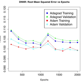
The performance of the Adagrad and Adam optimizers is illustrated in figure 3.
● ● ● ● ● ● ● ● ● ●
500
1000
1500
2000
0.090
0.095
0.100
0.105
0.110
0.115
0.120
DNNR: Root Mean Squared Error vs Epochs
Epochs
RMSE
●
Adagrad Training
Adagrad Validation
Adam Training
Adam Validation
Figure 3. Improvement in the performance of the DNN regressor, as measured by the RMSE, for
the Adam optimizer compared to the Adagrad optimizer. Sometimes instabilities during training are observed; usually they are overcome by running for a large number of epochs.
5 Discussion
To quantify the performance of the regressors, for each mass bin the “measured” forward-backward asymmetryAFBis extracted from the ensemble of all predictions for the events
asymmetries and the four true asymmetries (RMSEasym) is used as a measure of the
perfor-mance for each model training. This is compared to the traditional high energy physics way of doing the analysis by counting forward and backward events, and summarized in table 2.
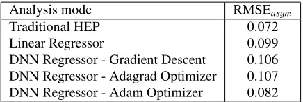
Table 2.Comparison of the performance of different regressors.
Analysis mode RMSEasym
Traditional HEP 0.072
Linear Regressor 0.099
DNN Regressor - Gradient Descent 0.106 DNN Regressor - Adagrad Optimizer 0.107 DNN Regressor - Adam Optimizer 0.082
Already the Linear Regressor is able to provide a decent performance after normalizing the input features. This improves further for the DNN Regressor when the Adam Optimizer is used. In contrast the Adagrad and Stochastic Gradient Descent Optimizers were not able to outperform the Linear Regressor in this feasibility study. The best performance with a Neural Net Regressor is starting to approach the traditional way of measuring the forward-backward asymmetry - the precision, as measured by RMSEasym, is only 14% worse, which is
an impressive result given the small size of the learning dataset. It is reasonable to expect that by increasing considerably the size of the simulated samples, the machine learning results can improve and be at least on par with the traditional approach.
6 Future Work
The results presented here are just the initial feasibility study. Next possible steps include:
• Substantially increase the size of the Monte Carlo samples
• Tune the hyperparameters of DNN for optimal performance
• The ultimate goal would be to perform a regression for the electroweak mixing angle di-rectly on the data; this would require analyzing millions or tens of millions of events.
7 Outlook
asymmetries and the four true asymmetries (RMSEasym) is used as a measure of the
perfor-mance for each model training. This is compared to the traditional high energy physics way of doing the analysis by counting forward and backward events, and summarized in table 2.
Table 2.Comparison of the performance of different regressors.
Analysis mode RMSEasym
Traditional HEP 0.072
Linear Regressor 0.099
DNN Regressor - Gradient Descent 0.106 DNN Regressor - Adagrad Optimizer 0.107 DNN Regressor - Adam Optimizer 0.082
Already the Linear Regressor is able to provide a decent performance after normalizing the input features. This improves further for the DNN Regressor when the Adam Optimizer is used. In contrast the Adagrad and Stochastic Gradient Descent Optimizers were not able to outperform the Linear Regressor in this feasibility study. The best performance with a Neural Net Regressor is starting to approach the traditional way of measuring the forward-backward asymmetry - the precision, as measured by RMSEasym, is only 14% worse, which is
an impressive result given the small size of the learning dataset. It is reasonable to expect that by increasing considerably the size of the simulated samples, the machine learning results can improve and be at least on par with the traditional approach.
6 Future Work
The results presented here are just the initial feasibility study. Next possible steps include:
• Substantially increase the size of the Monte Carlo samples
• Tune the hyperparameters of DNN for optimal performance
• The ultimate goal would be to perform a regression for the electroweak mixing angle di-rectly on the data; this would require analyzing millions or tens of millions of events.
7 Outlook
Machine learning techniques show interesting potential for precision measurements at the LHC. They are able to learn how to extract complex quantities like the forward-backward asymmetry of lepton pairs in proton-proton collisions at the LHC without much knowledge of the quite sophisticated underlying physics. Deep Neural Net regressors can outperform linear regressors helped by the introduction of synthetic features, as they are able to learn the non-linearities of the problem. The first results of this feasibility study look promising. It remains to be seen if ML techniques can outperform in precision the traditional analyses. This will be the focus of future exploration of this and similar topics.
References
[1] S. Haywoodet al., “Electroweak physics,” In Geneva 1999, Standard model physics (and more) at the LHC, 117-230 [hep-ph/0003275].
[2] J. C. Collins and D. E. Soper, Phys. Rev. D16, 2219 (1977). [3] T. Sjöstrand, S. Mrenna and P. Skands, JHEP0605, 026 (2006).
[4] T. Sjöstrand, S. Mrenna and P. Skands, Comput. Phys. Comm.178, 852 (2008). [5] T. Sjöstrandet al., Comput.Phys.Commun.191, 159-177 (2015).
[6] J. Pumplin, D.R. Stump, J. Huston, H.L. Lai, P. Nadolsky and W.K. Tung, JHEP0207, 012 (2002).
[7] V. Khachatryan et al. [CMS Collaboration], Eur. Phys. J. C 76, no. 6, 325 (2016), [arXiv:1601.04768 [hep-ex]].
[8] S. D. Drell and T. M. Yan, Phys. Rev. Lett.25, 316 (1970); Erratum: [Phys. Rev. Lett.
25, 902 (1970)].