Drift Chambers Simulations in BM@N Experiment

Drift Chambers Simulations in BM@N Experiment

Ján Fedorišin1,a

1_{Veksler and Baldin Laboratory of High Energy Physics, Joint Institute for Nuclear Research, 141980 Dubna,}

Moscow region, Russia

Abstract. Drift chambers constitute an important part of the tracking system of the BM@N experiment designed to study the production of baryonic matter at the Nuclotron energies. GEANT programming package is employed to investigate the drift chamber response to particles produced in relativistic nuclear collisions of C+C nuclei, which are simulated by the UrQMD and LAQGSM Monte Carlo generators. These simulations are combined with the first BM@N experimental data to estimate particle track coordinates and their errors.

1 Introduction

BM@N (Baryonic Matter at Nuclotron) [1] is a fixed target experiment at the JINR NICA-Nuclotron complex aimed to study the hot compressed nuclear matter produced in collisions of heavy nuclei with emphasis put on strange matter production. The BM@N physical program includes:

• study of strange and multistrange hadron production;

• in-medium properties of vector mesons;

• strangeness in elementary p+p and proton induced p+A reactions;

• exotics: multistrange nuclei, strange dibaryons, strangelets.

JINR Nuclotron is capable to accelerate heavy-ion beams with energies from 1 to 6 GeV per nucleon. Various nuclei with atomic numbers up to197_{Au are to be used as target or projectile nuclei}

−p, d, C, Cu, Xe, Au, etc. The test run in February – March 2015 has already provided first data with d, C and Cu beams on C, Cu targets. The xenon beam is planned for the end of 2017 and the gold beam is expected in 2018.

2 BM@N experimental layout

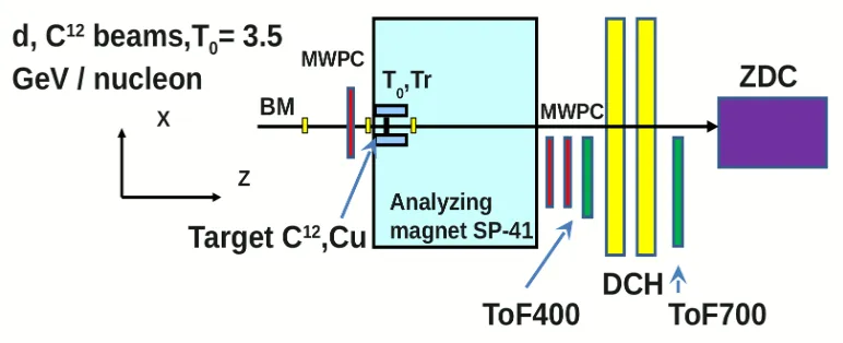
The first version of BM@N experimental set-up is outlined in Fig. 1.

The target is positioned at the front edge of the analyzing magnet. The Outer Tracker including two Drift Chambers (DCH) and three Multi-Wired Proportional Chambers (MWPC) is placed outside the magnetic field. In the future, the BM@N tracking system will be complemented with the Central

a_{e-mail: [email protected]} DOI: 10.1051/

C

Owned by the authors, published by EDP Sciences, 201

/20108 0 0 (201 ) epjconf

EPJ Web of Conferences , 0 0

1

610

6

6 8

2 2

2 2 1

1

Figure 1.BM@N experimental set-up for technical run in February-March 2015

Tracker consisting of Gas Electron Multiplier (GEM) coordinate detectors positioned inside the an-alyzing magnet. Two sets of Time of Flight (ToF) detectors are employed for particle identification. They are positioned “near to magnet” and “far from magnet” to identify hadrons and light nuclei with small as well as large momenta above 2 GeV/c. Zero Degree Calorimeter (ZDC) is installed at the far end of the experiment setup to measure the centrality of the nucleus-nucleus collisions as well as to form a trigger signal based on the properties of the deposited energy distribution.

3 Drift chambers

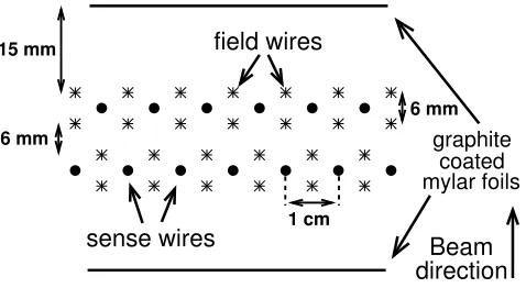
Two identical drift chambers reused from the NA-48 experiment at CERN [2] are suitable for ion beams with intermediate atomic numbers. They have octagonal shape with edge length 120 cm and fiducial area about 4.5 m2. The central aperture for the beam pipe has 12 cm radius. The drift chamber consists of 4 segments filled with 70/30 % mixture of Ar and CO2as a working gas. The DCH segment geometry is sketched in Fig. 2.

It contains two sensitive wire planes staggered by 0.5 cm with the anode wire pitch of 1 cm. Such configuration helps to resolve the left-right ambiguities of the detected particle tracks. Furthermore, each DCH segment measures different track coordinate in the transverse plane relative to the beam axis. This is achieved by the different azimuthal orientations of the DCH segments that are respec-tively rotated by anglesα=0◦,90◦,±45◦around the z axes in DCH local coordinate frames.

The principle of DCH operation is virtually the same as for any other gaseous coordinate detector utilized in high energy physics [3, 4]. Primary charge consisting of electron-ion clusters is left along a charged particle path in DCH gas volume. This charge subsequently drifts towards the electrodes, giving rise to an avalanche near the anode. Finally, the anode signal is generated, processed by the detector electronics and converted to a particle coordinate.

4 Simulations in BM@N experiment

graphite coated mylar foils

6 mm

6 mm 15 mm

1 cm

field wires

sense wires

_Beam

direction

Figure 2.Drift Chamber segment with anodes and field wires indicated by dots and asterisks respectively

At the first stage of the BM@N simulation-reconstruction chain, the collisions of relativistic heavy nuclei along with the production of secondary particles are simulated by UrQMD [5], QGSM [6] or LAQGSM [7] models. Then, passage of produced particles through the detectors, interactions with the detector materials and particle energy losses are simulated either by GEANT [8] or GARFIELD [9] programs. Eventually, the detector response, signal simulation and track hit production are imitated by GARFIELD and/or a special approach, depending on the type and specific characteristics of the employed detectors. Simulated data production and processing is often combined with input from real data, if available.

The presented method used for DCH hit estimation is based on LAQGSM C+C data at 4 AGeV.

5 Drift time to drift distance calibration

After GEANT simulates the DCH response to particles generated by LAQGSM, the next task is to reconstruct the particle tracks. However, in order to reconstruct DCH track coordinates, first we must estimate the distances of closest approach (DCA) of tracks to the anode wires, since DCA is not directly measured in the experiment. Instead, the drift time of the earliest electrons arriving on the anode wire is the available experimental observable.

The calibration method described in detail, e.g., in [10, 11] or [12] converts the measured drift times to DCAs.

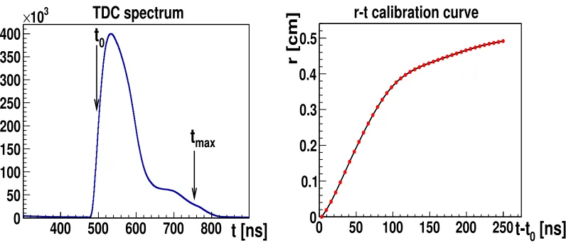
In the presented analysis, real drift time spectra (instead of simulated ones) are used because as already mentioned above the first BM@N experimental data with C+C collisions is already available. A typical drift time distribution measured in the experiment is shown in figure 3 on the left. First, it is necessary to estimate the minimum and maximum drift timest0 andtmax corresponding to the minimum and maximum drift distancesr0≈0 andrmax=0.5 cm.

This can be done for instance by fitting the drift time spectra with the empirical function described in [10, 11], or simply finding the inflection points indicating the positions of significant points in the experimental drift time distributions, includingt0andtmax.

If the DCA distribution is uniform, the isochronous radius-time relation is estimated by integrating the drift time spectrum:

r(t)= rmax

Ntot _t

0

dN dt dt

_{, (1)}

400

500

600

700

800

0

50

100

150

200

250

300

350

400

10

×

TDC spectrum

t [ns]

max

t

0

t

0

50

100

150

200

250

0

0.1

0.2

0.3

0.4

0.5

[ns]

t-t

r-t calibration curve

Figure 3.Experimental drift time spectrum for C+C collisions (left) and the correspondingr–tcalibration curve (right)

whereNtotis total number of hits and timetgradually increases in equidistant steps fromt0totmax. The resultingr-tcalibration curve obtained for our data is shown in figure 3, right panel. Typical electron drift velocities estimated from this curve are about 40μm/ns fort−t0100 ns and 20μm/ns fort−t0 100 ns.

6 Hit and track reconstruction

After estimating the measured track coordinates, there are still 4 more coordinates per DCH track left unknown. They are calculated using the information about the shape of the particle tracks.

In the absence of the magnetic field in both DCHs it is reasonable to approximate the tracks by straight lines defined by the intersection points with four DCH planes:

x1, y1, z1, x2, y2, z2, u1(x3, y3), u2(x3, y3), z3, v1(x4, y4), v2(x4, y4), z4,

wherey1,x2,u2,v2are measured DCH coordinates andz1,z2,z3,z4are defined by the DCH geometry and position. The measured coordinatesu2,v2in the last two DCH planes, rotated by the angles±α, are defined by the equations:

u2=y3cos(α)−x3sin(α), v2=y4cos(−α)−x4sin(−α)=y4cos(α)+x4sin(α), (2)

whereα=45◦. The rotated coordinatesu1,v1are neither measured nor needed in our next calculations therefore from now on we use the denotationu2→uandv2→v.

All the coordinates are bound together by the system of linear equations:

x2−x1

z2−z1 =

x3−x1

z3−z1 =

x4−x1

z4−z1,

y2−y1

z2−z1 = y3−y1

z3−z1 = y4−y1

z4−z1,

(3)

which is solved for the unknown coordinatesy2,x1,x3,y3,x4,y4. The found track coordinates are:

x1=

v/cosα−y1 z4−z1 −

u/cosα−y1 z3−z1 −

2x2tanα z2−z1

1

z4−z1 +

1

z3−z1 −

2

z2−z1

tanα ,

y2=(x2−x1) tanα+(x1tanα−y1+u/cosα)·z2−z1

z3−z1

+y1, (5)

y3=(y2−y1)·z 3−z1

z2−z1 +y1, x3=

y3−u/cosα

tanα , (6)

y4=(y2−y1)·z 4−z1

z2−z1

+y1, x4 =

y4−v/cosα

−tanα . (7)

Each drift chamber produces minimal information to define a linear track candidate.

7 Results and consistency checks

Finally, the track candidates from both drift chambers are combined to produce the global track can-didates. Their straight line fits are used to increase the precision of the estimated track geometry parameters as well as to get rid of the combinatorial background.

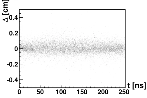
Track hit reconstruction quality and consistency checks based on our fit results are presented in figures 4 and 5. Figure 4 shows the dependence of the hit residuals

Δ =|rfitted−ranode| − |rmeasured−ranode| (8)

on the drift timet =t−t0, providing that the substitute symbolrrepresentsy,x,u,vcoordinates in all the four DCH planes respectively.

0

50

100

150

200

250

-0.4

-0.2

0

0.2

0.4

[cm]

Δ

t [ns]

Figure 4.Hit residualsΔas function of DCH drift timet

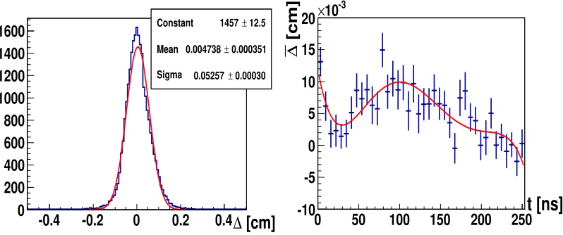
Figure 5 left presents the projection of the previous plot on theΔaxis. Its Gaussian fit indicates a DCH hit coordinate resolutionσ ≈ 500μm. Average residuals ¯Δvs DCH drift time are shown in the figure 5 right panel. They suggest systematic uncertainties of ther–tcalibration curve. This information can be later used to correct the calibration curve by minimizing the hit residuals.

Constant 1457 ±12.5

Mean 0.004738 ± 0.000351

Sigma 0.05257 ± 0.00030

-0.4

-0.2

0

0.2

0.4

0

200

400

600

800

1000

1200

1400

1600

Mean 0.004738 ± 0.000351

Sigma 0.05257 ± 0.00030

[cm]

Δ

-10

0

50

100

150

200

250

-5

0

5

10

15

20

-3

10

×

t [ns]

[cm]

Δ

Figure 5.DCH hit residualsΔ(left) and the average residuals ¯Δas a function of DCH drift time (right)

8 Summary

1. The BM@N drift chambers geometry was programmed using the ROOT geometry package.

2. This geometry setup along with LAQGSM [7] and GEANT [8] was used to simulate the condi-tions of BM@N experiment.

3. The experimentalr–tcalibration curve was applied to calculate DCH hit coordinates.

4. DCH hits were estimated under the assumption of track linearity.

5. The DCH hit residual spectra indicate a preliminary coordinate resolutionσ ≈500μm and a systematic bias ofΔup to 100μm. Minimizing this bias by the autocalibration method [10–12] should result in significant improvement ofσ.

References

[1] T.O.Ablyazimov et al., BM@N Collaboration,BM@N – Baryonic Matter at Nuclotron (Con-ceptual Design Report), http://nica.jinr.ru/files/BM@N/BMN_CDR.pdf (2012)

[2] D. Béderéde et al., Nucl. Instrum. Meth.A 367, 88–91 (1995)

[3] F. Sauli,Gaseous Radiation Detectors, (Cambridge Monographs on Particle Physics, 2014) [4] W. Blum, W. Riegler, L. Rolandi, Particle Detection with Drift Chambers, (Springer-Verlag

Berlin Heidelberg, 1993)

[5] S. A. Bass et al., Prog. Part. Nucl. Phys.41, 225–370 (1998)

[6] N.S, Amelin, L.V. Bravina, L.N. Smirnova: Sov. J. Nucl. Phys.52, 362 (1990) [7] S.G. Mashnik et al., Advances in Space Research34, 1288–1296 (2004) [8] S. Agostinelli et al., Nucl. Instrum. Meth.A506, 250–303 (2003) [9] R. Veenhof, http://garfield.web.cern.ch/garfield/

[10] G. Avolio et al., Nucl. Instrum. Meth.A 523, 309–322 (2004) [11] W. Erni et al., Eur. Phys. J.49: 25 (2013)