Grazing incidence scattering

(1)

JDN 23

Grazing

incidence

scattering

MaxWolff

DepartmentforPhysicsandAstronomy,UppsalaUniversity,75120Uppsala,Sweden

Abstract.Reflectometry experiments probe the scattering length density along the

nor-mal of interfaces by analysing the specularly scattered intensity. Lateral fluctuations result in intensity scattered away from the specular condition. In this paper the principles and peculiarities of grazing incidence scattering experiments are explained. One specific example, the self assembly of polymer micelles close to interfaces, is taken as a show case in order to introduce the scattering geometry and accessible length scales. The basic idea of the distorted wave Born approximation is lined out and some scientific examples are summarized.

1 The importance of surface effects

With the development and miniaturization of modern technology the need for advanced experimen-tal methods in surface science has increased tremendously. This fact is reflected, for example, by the development of atomic probes [1] or electron microscopy [2]. In the field of x-ray and neutron scattering the number of reflectometers, which are most relevant for surface science, is growing and with the years specular reflectometry measurements have become a routine tool to extract the density profiles of materials across interfaces with almost atomic resolution (see chapter 04001 by F. Cousin and A. Chenneviere). A list of neutron reflectometers as well as relevant citations describing those can be found in Ref. [3] and an introduction in reflectometry and grazing incidence is found in [4]. However, specular reflectivity measurements can only reveal the scattering length density (SLD) pro-file across an interface with the scattering potential averaged in the plane of the interface and over the coherence volume of the beam. To become more specific, inter-diffusion and roughness or even

regular patterns on a surface can not be characterized (see Figure 1). In the case of roughness lateral correlations in the plane along the interface may be present. These give rise to interferences and a modulation of the scattered intensity. The lateral correlations can be extracted from so called off

-specular (OFFSpec), grazing incidence small angle scattering (GISAS) or diffraction (GID). During

the last 15 years most neutron reflectometers have become equipped with position sensitive detectors allowing an efficient collection of OFFSpec and grazing incidence scattering (GIS) data. Still the

method is not exploited to its full potential, which results on the one hand from the fact that easy to use and robust fitting routines are not yet developed and on the other hand from the strongly limited flux and dynamic range on neutron instruments. Typically, OFFSpec and GIS intensities are three or more orders of magnitude lower in intensity than their specular counterparts.

(2)

Nb. yellow

7 5 2 0

10

Interdiffusion Roughness

Figure 1. Roughness and inter-diffusion: In the left panel a continuous line can be drawn between the two

materials, whereas in the right panel isolated islands exist. The integrated number of yellow and blue circles along the horizontal direction is the same. Specular reflectivity can not distinguish between the two scenarios.

This manuscript is structured as follows: First the scattering geometry and the peculiarities of OFF-Spec and GIS is explained on a specific example of polymer micelles self assembling at a solid bound-ary. Then the distorted wave Born approximation (DWBA) is outlined and finally some scientific examples are presented.

1.1 Scattering geometry

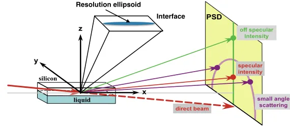
The scattering geometry in neutron reflectometry (NR) is usually defined in cartesian coordinates with the z direction along the normal of the interfaces. The x-direction is in the scattering plane and y is perpendicular to x and z (see Figure 2). In the case of a buried liquid interface a neutron beam may pass trough a silicon wafer, get scattered at the solid-liquid boundary and detected by an area detector. Note, since the absorption of neutrons in silicon is low and the scattering potential of deuterated liquids is large, such experiments can be performed in a straight forward way with a minimum loss in flux and a critical momentum transfer of total external reflection present.

The intensity scattered at the same incident and exit angles (orange arrows in Figure 2) is the specular reflectivity and contains the information about the SLD profile along the surface normal. Intensity scattered at different exit angles but still in the scattering plane (symbolized green) is usually called

OFFSpec and intensity registered for exit angles out of the scattering plane is small angle scattering (SAS). The three components of the scattering vector Q, along the x, y and z-direction, are calculated

Interface Resolution ellipsoid

(3)

3 JDN 23

0.001 0.01 0.1 1

Reflectivity

0.05 0.04 0.03 0.02 0.01

Qz (A-1)

Measurement

RF 0.001

0.01 0.1 1

Reflectivity

0.05 0.04 0.03 0.02 0.01

Qz (A-1)

Measurement RF

Hydrophilic interface Hydrophobic interface

-2 -2

-10 -10

1 1

2 2

Intensity (10

-2 I

0

)

-1.0 0.0 1.0

(degree)

p

log(D ) ( m)

0 1 2

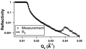
Figure 3. Reflectivity data taken with a micellar polymer solution in the liquid phase in contact with a silicon

wafer compared to the Fresnel-reflectivityRF.

as follows:

Qx = 4π

λ

cosαfcosφ−cosαi

(1)

Qy = 4π

λ sinφ (2)

Qz = 4π

λ

sinαi+sinαf

(3)

withαiandαf the angle of the incident and exiting beam with respect to the sample’s surface,λthe

wavelength andφthe scattering angle out of the scattering plane.

2 Block-polymers and micelles

In the following the peculiarities of grazing incidence small angle neutron scattering (GISANS) and OFFSpec will be explained on one specific example, namely aqueous solutions of block polymers and their assembly at the solid-liquid boundary. This system offers a strong scattering signal on

all length scales relevant for GIS experiments. In aqueous solution the molecules tend to form micelles (self-aggregartions of molecules). Depending on temperature and volume fraction these may form liquid or crystalline phases. The sample is a 18.5 % (in weight) solution of Pluronic F127 (EO99-PO65-EO99) in deuterated water providing a good contrast for neutrons. The bulk properties of such samples are known in great detail [6, 7]. In the case of F127 face centred cubic (fcc) crystals are formed at elevated concentrations or temperatures.

Figure 3 shows the specular reflected intensity taken with the sample in a liquid phase at 295 K compared to the Fresnel-reflectivity. The data is corrected for the SAS by substracting the intensity for a detector off-set angle, from the specular condition, of 0.3◦. AtQz = 0.04 Å, the intensity is

increased. This Bragg peak indicates several layers of adsorbed micelles at conditions, which are still in the liquid phase with no fcc structure present in the bulk.

3 Off-specular and GISANS

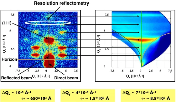
In the crystalline phase (temperature 298 K) a fcc dense packed structure is formed. Figure 4 (left panel) represents a GISANS pattern collected on an area detector for a monochromatic incident beam impinging the sample under an incident angleαiclose to the critical angle of total external reflection

(4)

ΔQx ~ 10-5 Å-1

⇔ ~ 650*103 Å

Qz

[10

-2 Å -1]

7.5

2.5 5

0

0 -2.5 2.5 5

-5 7.5

-7.5

Qx [10-4 Å-1] Qz

[10

-2 Å -1]

7.5

2.5 5

0

0 -2.5 2.5 5

-5 7.5

-7.5

Qy [10-2 Å-1]

ΔQy ~ 4*10-3 Å-1

⇔ ~ 1.5*103 Å ΔQz ~ 7*10

-4_Å-1

⇔ ~ 8.5*103 Å

Direct beam Reﬂected beam

Horizon (111)

Resolution reﬂectometry

Figure 4.Scattering patterns for a micellar crystal in contact to a silicon wafer. The panel on the left hand side depicts the GISANS pattern form the cubic close packed structure. The panel on the right hand side depicts reflectometry data (specular and OFFSpec) from the same sample but with a relaxed resolution along the y-direction [5].

for a drop of 1/e of the incident intensity). αcfor a neutron wavelength of 0.44 nm is 0.25◦and

de-fined by the SLD of silicon and the polymer solution. For no momentum transferQ =0 the direct

beam hits the detector at the very bottom in the middle. Slightly above the reflected beam is visible. Half way between these two peaks the sample horizon (brown line), dividing intensity transmitted by and reflected at the interface, is found. Clearly below the horizon the intensity is low (dark blue region below Qz =0.01 Å−1) due to the enhanced absorption or incoherent scattering inside of the

liquid sample as well as of the sealing of the liquid cell [10]. Note: the image shows raw data andQz

was not corrected for refraction effectsQz,in =

Q2

z−Q2c, withQz,in theQzvalue inside the liquid.

All other reflections are Bragg peaks resulting from a cubic dense packing of the polymer micelles close to the solid interface [11]. The projection of the resolution on the x, y and z axis for GIS is dependent onαiand the exit angleαf, since the coordinate system is fixed to the sample and not to

the instrument [5]. Specifically, for this example andQ=0.04 Å−1_{the resolution}_Q_x₌₁₀−5 _Å−1_is determined by the pixel size of the detector and the scattering angle. The resolutionQy=4×10−3Å−1 andQz=7×10−4Å−1is given by horizontal and vertical slits. In real space the resolution is defined

by the coherence volume of the beam projected onto the respective axis of the coordinate system and is roughly 65µm, 150 nm and 850 nm along the x, y and z-direction, respectively, for the incident beam angle of 0.3◦_.

On the monochromatic instrumentαiandαf are changed and for each setting and an image, similar to

the one shown in the panel on the left hand side, is detected. The panel on the right hand side (Fig. 4) shows the result of such a NR measurement, including the OFFSpec scattering. In this representation the horizon is again represented by a brown line. The two panels on the left and right (Figure 4) are orthogonal but intersect along the black lines. This line is almost identical with the sample horizon in the right panel. Due to the non-linear transformation of the coordinateQxthe black line is curved in

the panel on the right hand side.

(5)

5 JDN 23

Intensity

-1.5 -1.0 -0.5 0.0 0.5 1.0 1.5

αi - αf [degree]

0 0.5 1 1.5

0 0.5 1 1.5 2 2.5 3 3.5

Incident beam angle [°]

Scattering angle [°]

0 0.5 1 1.5 2 2.5 3

Horizon

Specular r

eﬂectivity

Bragg

log(Intensity) [arb. units] 0.0 0.1 0.2Q [nm-10.3] 0.4 0.5 Reﬂectivity

Background Reﬂectivity corr.

Bragg reﬂection

log(Intensity) [arb. units]

(111) peak Specular

Diﬀuse

Horizon Horizon

Figure 5. Left panel: Rocking scan for the sample in the crystalline phase at Qz =0.38 nm−1. Right panel: Correction of the specular scattered intensity for SAS.

Qy0 is detected in the Qx, Qzplane. In order to extract the true specular reflectivity this contribution

has to be corrected for, since the intensity is not scattered specular but appears in the specular direc-tion. This is a severe challenge for samples with strong SAS, when the SAS can be equal or stronger than the specular signal. Figure 5, right panel, demonstrates this effect [20]. The detected specular

NR is plotted on a logarithmic scale versusQz (circles marked with a cross). The background, for

an offset ofαiandαf of 0.25◦, is represented by open circles. ForQz >0.2nm−1the reflectivity is

dominated by SAS and the true specular signal (black dots) can hardly be extracted with statistical significance.

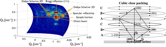
The panels on the right and left hand side, Fig. 6, illustrate the unit cell of the cubic close packing and the GISANS plotted as color map onto the Ewald sphere, respectively. The detector plane represents a curved surface with Q=0 at the position of the direct beam. The second and only other point where the

in-plane coordinatesQxandQyare zero is the point where the specular scattered intensity is detected.

All other points on the detector have none-zeroQxand/orQycomponents.

Considering a densely packed cubic structure at the interface, the (111) lattice planes are parallel to the solid-liquid boundary and the Bragg reflections resulting from them should have no in-plane component (Qx=Qy=0). This implies that the (111) reflection can only be detected in a GISANS

Qy [nm-1]

Qz [nm-1]

Qx [nm-1]

Direct beam Specular reﬂectivity Bragg reﬂection (111)

Sample horizon 1

-0.5 0.5

0

-0.5

0.5 ₀

-1 -0.1 -0.05 0

0.05 -1

1

Debye Scherrer 2D Debye Scherrer 2D

FIG. 3. Detector image for a fcc crystalline structure plotted as color map on the surface of the

Ewald sphere.

y and z is defined with respect to the sample surface as shown in Figure 1. A more detailed

discussion of the length-scales probed along the di↵erent directions can be found in24_{. It is}

clear that the detector plane represents a curved surface with Q=0 at the position of the

direct beam. The second and only other point where the in-plane coordinatesQxandQy

are zero is the point where the specular scattered intensity is detected. All other points on

the detector have none-zeroQxand/orQycomponents.

Considering a densely packed cubic structure at the interface, the (111) lattice planes would

be parallel to the solid-liquid boundary and the Bragg reflections resulting from them should

have no in-plane component (Qx=Qy= 0). This implies that the (111) reflection can only

be detected if it has a certain rocking width along Qx. The values probed along theQx

direction are much smaller than those probed alongQyandQzand for a crystal coherence

on the order ofµm a finite intensity is detected in the detector plane. Moreover with

de-creasing wavelength the momentum transfer along the x direction decreases at the position

of the Bragg refelection for small Q20_{. This implies that for a specific crystal coherence the}

intensity scattered into the detector plane should increase with decreasing wavelength. All

other four Bragg reflections are only visible if the crystalline structure is a two dimensional

powder with respect to the sample interface24_{, since the}_Qy _{values are much larger than}

theQxvalues and the probability of a crystal orientation with the Bragg reflection on the

Ewald sphere is unlikely. Moreover, for a single crystal arrangement the reflections with and

without prime visible in figure 2 can never be detected on the Ewald sphere at the same

time, since they would be separated by an angle of 180 on the Debye-Scherrer ring, which

Q

Q (000)

Q

(004)

(002) (022)

(222)

Hydrophilic surface

A B C A B C

Hydrophobic surface−y

Q (000)

(222) (004)

(111) (002)_hcp

hcp

Qz

Qx

A B A B

(113)_hcp

(111)_hcp hcp

hcp

z

hcp (200)

(311)

(111)

z

y (000) (−111)

Cubic close packing Hexagonal close packing Ewald−sphere

(6)

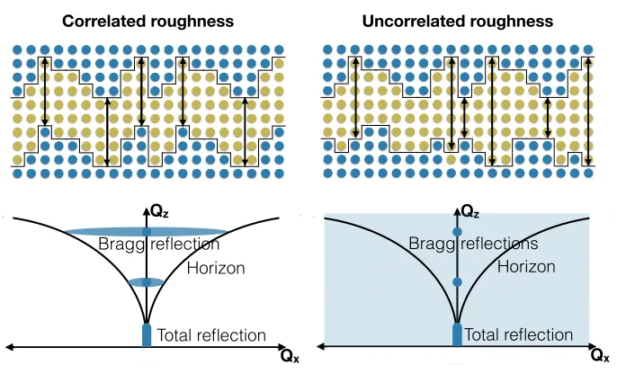
Correlated roughness Uncorrelated roughness

Qz

Qx

Horizon

Total reﬂection Bragg reﬂection

Qz

Qx

Horizon

Total reﬂection Bragg reﬂections

Figure 7. Structure and off-specular scattering from rough surfaces for perfectly correlated (left panels) and

uncorrelated (right panels) interfaces.

experiment if it has a certain rocking width along Qxor in other words correlated roughness of the

micellar layers is present. All other four Bragg reflections are only visible if the crystalline structure is a two dimensional powder with respect to the sample interface [5], since the Qy values are much

larger than theQxvalues and the probability of a crystal orientation with the Bragg reflection on the

Ewald sphere is unlikely.

The (111) reflection at Qz ≈0.38 nm−1 andQy = 0 is smeared out in the reflectivity measurement

(right panel) along Qxdue to correlated roughness. Figure 5, left panel, represents a cut along this

reflection along Qx. Such a cut is called Rocking curve, theαiandαf are scanned for given scattering

angle (see x-axis in Figure 5, left panel). The narrow component is the specular scattered intensity and reflects long range orientational correlations over the coherence volume of the neutron beam [21], indicated by the ellipsoid in Fig. 2 (resolution ellipsoid). The broad component is related to diffuse or

OFFSpec scattering and results from the finite lateral correlations of the SLD fluctuations contributing to the Bragg peak along the plane of the interface. As mentioned the length scale probed along the x-direction is about two orders of magnitude larger than the one probed along y and z (see Figure 4). The GISANS together with an analysis of the width of the (111) reflection in the off-specular

scattering regime can be used to analyse the texture as well as the size of the micellar crystallites [16]. Figure 7, left and right panel, depicts the extreme cases of perfectly correlated and uncorrelated inter-face roughness, respectively, and the resulting OFFSpec scattering. For a perfectly correlated rough-ness (left panels) between layers the OFFSpec scattering becomes concentrated along so called Bragg sheets, showing up as horizontal lines at a certainQzand running alongQx. The width of the sheets

is the reciprocal lateral correlation length. For uncorrelated layers the OFFSpec scattered intensity is smeared out over the whole Q space. Note, the discussion above is based on kinematic approxima-tions and neglects the dynamic effects which can be important in reflectometry experiments. However,

dynamical effects (apart from total reflection) are typically important for very well ordered samples,

(7)

7 JDN 23

The main interest for neutron mirrors is to achieve high reflectivity. For this reason we focus to the specular reflectivity in the region of the first Bragg reflection (Fig. 2). The results of series A2 are consistent with series A1. It turns out that fortCr¼4 ˚A the intensity increases by approximately 3%, and for tCr¼8 ˚A it decreases by approximately 5%.

Based on these results we expect to achieve higher reflectivities for SM and ML monochromators. The layer thicknesses are calculated using the formalism of Hayter [7].Fig. 3shows the reflectivities of series B, Ti/Cr/Ni/Cr

m¼2 supermirrors with 60 Ti/Ni periods and Cr inter-layers withtCr¼028 ˚A at every interface. The Cr-less SM shows a reflectivity of 0.91 at m¼2. The use of Cr interlayers increases the reflectivity up to 0.93 fortCr¼2 ˚A and 3 A˚. A further increase of the Cr interlayer thickness leads to a decrease of the reflectivity: 0.92 fortCr¼4 ˚A, 0.91 for 5 A˚, and 0.87 for 6 A˚ and 8 A˚ oftCr. These results are consistent with the observations from the multilayers of series A, where diffusion barriers in the range of a closed monolayer lead to a rise of intensity. However, when the interlayer thickness is larger than the interdiffusion layer between Ni and Ti (E6 A˚) the benefit of the Cr interlayers is lost and the reflectivity even decreases. The application of Cr interlayers at every boundary for supermirrors with 200 layers and more could not show an improvement of the reflectivity up to this day. We think, this is due to the fact that the higher roughness due to the larger number of layers prohibits the growth of closed Cr layers with thicknesses of 2–4 A˚ (only a fraction of the surface is covered with Cr). We suppose that this leads to a negative effect because of interdiffusion of Ni and Ti and a variation ARTICLE IN PRESS

0.20

0.15

0.10

0.05

0

-0.05 0.05

Transmitted beam Yoneda

RDS Bragg like

sheet

4

3

2

1

0

ki-kf ki

+kf

0.20

0.15

0.10

0.05

0

-0.05 0.05

4

3

2

1

0

ki-kf ki

+kf

0.20

0.15

0.10

0.05

0

-0.05 0.05

4

3

2

1

0

ki-kf ki

+kf

SL Bragg peaks

(a)

(b)

(c)

Fig. 2. Two-dimensional intensity maps of the scattering from a [Ti(70 A˚)/

Cr (tCr)/Ni(70 A˚)/Cr (tCr)]20multilayer plotted as function ofki+kfandki

-kf., with Cr interlayer thicknesses of (a) 0, (b) 4, and (c) 8 A˚.

0.00 0.02 0.04 0.06 0.08 0.10

f0ÅCr(x) f3ÅCr(x)

Intensity [a. u.]

qz [Å-1]

Cr m=2

interlayer & reflectivity 0Å 91% 2Å 93% 3Å 93% 4Å 92% 5Å 91% 6Å 87% 8Å 87%

Fig. 3. Reflectivity of a series of Ti/Cr/Ni/Crm¼2 supermirrors with 60

Ti/Ni periods and Cr interlayers at every interface withtCr¼028 ˚A. The

data are shifted for clarity.

M. Ay et al. / Nuclear Instruments and Methods in Physics Research A 562 (2006) 389–392 391

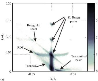
Figure 8.Two-dimensional intensity maps of the scattering from a [Ti(70 Å)/Ni(70 Å)]20multilayer plotted as

function ofki+kf andki−kf [12].

Still dynamic effects resulting in so called Yoneda and resonant diffuse scattering (RDS) will be

discussed briefly below. For illustration Fig. 8 depicts a scattering pattern collected with a TiNi mul-tilayer with 20 repetitions [12]. The intensity is plotted overki+kf andki−kf instead ofQxandQz

to avoid the compression of the scattering pattern close to the critical momentum transfer, resulting from the non-linear transformation to Q [13]. Yoneda scattering [14] results from an constructive in-terference of the incoming and outgoing wave field at the critical momentum transfer of total external reflection and enhances scattering from roughness along so called Yoneda wings (sample horizon). In addition, since the incident or exiting wave impinges under the critical momentum the scattering pattern gets distorted close to the horizon. This results in an upturn (towards larger Qzvalues) of the

Bragg sheets in this region. For multilayers there is additional interference of the waves scattered at each interface and again for constructive interference roughness scattering is enhanced resulting in RDS or Holy scattering [15].

4 Modes of measurement

As described in the previous chapters neutron scattering experiments can be done in two modes. The classical way are monochromatic instruments with a continuous flux of neutrons. For each point in Qthe scattering angle as well as the incident angle is chosen with respect to the sample, see Figure 9, bottom panel. For the time of flight (TOF) method a pulsed neutron beam is used with a polychro-matic beam and the wavelength is extracted from the time of flight of the neutron from the source to the detector. With this method a range of momentum transfers is measured for one given setting of the instrument, see Figure 9, top panel.

As a result a whole range of Q values around Qcand a range of penetration depth from the boundary

can be probed. For a momentum smaller than Qcthe penetration depth is small, on the order of 20

(8)

Q

kf

ki

Source

Monochromator Set of choppers

Neutron guide

Collimating slits

Collimating slits (specular reﬂectivity)

Detector (position sensitive for off-specular and grazing incidence) Source

Neutron guide

Collimating slits Collimating slits (specular reﬂectivity)

Detector (position sensitive for off-specular and grazing incidence)

Q k

i

k f Inciden

t beam Chopper Spin

flipper

A_nalyz er Exiting beamD_et

ec tor Sample

Collima tor Collima

tor

Sour ce Polar

izer

Spin flipper

Q

k i

k f Inciden

t beam

Chopper

Spin flipper

Analyz er

Exiting beam Det

ec tor

Sample

Collima tor

Sour ce

Polar izer

Spin flipper

Q k i

k f Inciden

t beam

Chopper

Spin flipper

Analyz er

Exiting beam Det

ec tor

Sample

Collima tor

Sour ce

Polar izer

Spin flipper

Q k_i

k_f Inciden

t beam Chopper Spin

flipper

Analyz er Exiting beamDetector Sample

Collima tor Collima

tor

Sour ce Polar

izer

Spin flipper

Q

kf

ki

Figure 9.Modes for reflectometry experiments, the top panel shows time of flight or polychromatic instruments

and the bottom panel monochromatic ones. On polychromatic instruments a range ofQvalues is probed for one

setting of the instrument.

micrometers, which is typical for neutrons. The height of the jump at the critical momentum is related to the extinction properties of the material. The curve shown in Figure 10 is calculated for the silicon-polymer solution interface discussed above. The incoherent scattering cross section is included in the absorption and extinction related to scattering is neglected. It is seen that the penetration depth into the liquid changes by four orders of magnitude within 10 % above and belowQc.

This implies that taking independent data in regions 1, 2 and 3 and achieving depth resolution is ex-tremely challenging since an excellent ∆Q

Qc is needed. In particular any tails of the resolution function

k

Sample Silicon

Position−Sensitive Detector

k

z

x y

3 1 2

101 102 103 104 105

Pen. depth [nm]

2.0 1.8 1.6 1.4 1.2 1.0 0.8 0.6

Q [Q/QC]

(9)

9 JDN 23

will immediately result in neutrons penetratingµm into the liquid and can dominate the scattering pat-tern [17]. ∆Q

Q is calculated by the following equation taking into account the wavelength distribution ∆λand a angular divergence∆θ:

∆Q

Q =

∆λ

λ 2

+(∆θcotθ)2 (4)

For small anglesθthis can be simplified:

∆Q

Q =

_∆_λ

λ 2

+

∆θ

θ 2

(5)

The most efficient use of neutrons is achieved for equal relative resolutions regarding wave length

and divergence. For a time of flight instrument the wavelength resolution is given by the length of the instrument, the time resolution of the detector as well as by the neutron pulse length and for a monochromatic instrument by the mosaic of the monochromator and the divergence in the neutron guide or the specifications of the velocity selector. The divergence of the beam can be adjusted on both types of instruments by slits. Let us assume a wavelength and angular resolution of 1 %. Regard-ing the wavelength this can easily be reached with time of flight methods or monochromators. For the angular resolution at a critical angle of 0.2◦_{a 1 % resolution implies a divergence of 0.002}◦_{or two}

pinholes of 1 mm diameter at a distance of almost 30 m. In addition the footprint of e.g. 0.175 mm for a 5 cm sample under the angle of 0.2◦_{is small.}

Figure 11 depicts patterns of intensity measured on SANS-2D (Rutherford Institute, Didcot, England) for the polymer solution discussed above but now in contact to two silicon wafers with distinct surface energies [18]. The incident beam was collimated to provide a divergence of 0.29◦ _{and 0.04}◦ _{along y}

and z direction, respectively. The incident beam angle was chosen to be 0.3◦ _{resulting in a critical}

wavelength for total external reflection ofλc=5.4 Å.

The three pictures for the hydrophilic silicon surface treated with piranha (top panels) and the hy-drophobic one coated with octadecyltrichlorosilane (OTS) (lower panels) were taken simultaneously for one incident beam angle with a fixed detector angle. The left panels correspond to the integration of the detector images for wavelengths ranging from 6-15.6 Å resulting in a penetration depth of the neutron beam into the polymer solution of approximately 10 nm (region 1 in Figure 10). The intensity integrated for short wavelengths of 1.75-5 Å and thus a large penetration depth of about 30µm is de-picted in the right panels. The central column summarizes the intensities for wavelengths integrated around the critical wavelength, 5-6 Å, resulting in an intermediate penetration depth of about 10µm. For the smallest penetration depth of about 10 nm a ring of scattered intensity is visible around the direct beam (Q=0) for the hydorphobic substrate. This ring is absent for the micelles in contact with

the hydrophilic surface. Note, the presence of the 111 reflection for these wavelength demonstrates the limited depth sensitivity of the measurement, since the constructive interference arises from lay-ers separated by more than 10 nm [17]. The difference in the intensity distribution for the sample

in contact to one or the other solid substrate becomes more pronounced for larger penetration depths (middle panels). At least ten Bragg reflections can be distinguished with the sample in contact to the hydrophilic surface, whereas still the ring of scattered intensity is dominant for the hydrohpobic one. For the largest penetration depth (right panels) both detector images are almost identical, reflecting the bulk structure and a vanishing influence of the interface.

(10)

EPJ Web of Conferences 188, 04002 (2018) https://doi.org/10.1051/epjconf/201818804002 JDN 23 Qz [nm -1] Qz [nm -1]

Qy [nm-1]

0.5

-1 - 0.5 0 1 -1 - 0.5 0 0.5 1

0.5

-1 - 0.5 0 1 Intensity [arb

. units] Intensity [arb . units] 0.5 1 0 0.5 1 0

Hydrophobic

~ 10 nm (< 1 µm) ~ 10 µm > 30 µm

1 0 4 2 3 1 0 4 2 3

Hydrophilic

(111) (111) (111)

(111) (111) (111) (222) (222) (222) (222) (200)’ (-111) (-311) (022) (311)’ (-111)’(200) (022)’ (311) (3-11) (-220) (2-20)

qyin ˚A1

qz

in

˚ A

1

-0.1 -0.05 0 0.05 0.1

2.5 3 3.5 4 4.5 0 0.05 0.1

(a) Hydrophobic wafer,l=2.55±0.03 ˚A

qyin ˚A 1

qz

in

˚ A

1

-0.1 -0.05 0 0.05 0.1

2.5 3 3.5 4 4.5 0 0.05 0.1

(b) Hydrophilic wafer,l=2.55±0.03 ˚A

qyin ˚A1

qz

in

˚ A

1

-0.1 -0.05 0 0.05 0.1

3.5 4 4.5 5 5.5 6 0 0.05 0.1

(c) Hydrophobic wafer,l=3.567±0.001 ˚A

qyin ˚A 1

qz

in

˚ A

1

-0.1 -0.05 0 0.05 0.1

3.5 4 4.5 5 5.5 6 6.5 0 0.05 0.1

(d) Hydrophilic wafer,l=3.567±0.001 ˚A

qyin ˚A1

qz

in

˚ A

1

-0.1 -0.05 0 0.05 0.1

3.5 4 4.5 5 5.5 6 0 0.05 0.1

(e) Hydrophobic wafer,l=4.583±0.001 ˚A

qyin ˚A 1

qz

in

˚ A

1

-0.1 -0.05 0 0.05 0.1

3.5 4 4.5 5 5.5 6 6.5 0 0.05 0.1

(f) Hydrophilic wafer,l=4.583±0.001 ˚A

qyin ˚A1

qz

in

˚ A

1

-0.1 -0.05 0 0.05 0.1

3 3.5 4 4.5 0 0.05 0.1

(g) Hydrophobic wafer,l=5.6±0.05 ˚A

qyin ˚A 1

qz

in

˚ A

1

-0.1 -0.05 0 0.05 0.1

3.5 4 4.5 5 5.5 6 0 0.05 0.1

(h) Hydrophilic wafer,l=5.6±0.001 ˚A

Figure 17: Data above the crystallization temperature evaluated at different wavelengths. Several peaks are visible.

30

qyin ˚A1

qz

in

˚ A

1

-0.1 -0.05 0 0.05 0.1

2.5 3 3.5 4 4.5 0 0.05 0.1

qyin ˚A1

qz

in

˚ A

1

-0.1 -0.05 0 0.05 0.1

2.5 3 3.5 4 4.5 0 0.05 0.1

qyin ˚A1

qz

in

˚ A

1

-0.1 -0.05 0 0.05 0.1

3.5 4 4.5 5 5.5 6 0 0.05 0.1

qyin ˚A1

qz

in

˚ A

1

-0.1 -0.05 0 0.05 0.1

3.5 4 4.5 5 5.5 6 6.5 0 0.05 0.1

qyin ˚A1

qz

in

˚ A

1

-0.1 -0.05 0 0.05 0.1

3.5 4 4.5 5 5.5 6 0 0.05 0.1

qyin ˚A1

qz

in

˚ A

1

-0.1 -0.05 0 0.05 0.1

3.5 4 4.5 5 5.5 6 6.5 0 0.05 0.1

qyin ˚A1

qz

in

˚ A

1

-0.1 -0.05 0 0.05 0.1

3 3.5 4 4.5 0 0.05 0.1

qyin ˚A1

qz

in

˚ A

1

-0.1 -0.05 0 0.05 0.1

3.5 4 4.5 5 5.5 6 0 0.05 0.1

30 4 Data visualization and evaluation

qyin ˚A 1

qz

in

˚ A

1

-0.1 -0.05 0 0.05 0.1

2.5 3 3.5 4 4.5 0 0.05 0.1

qyin ˚A 1

qz

in

˚ A

1

-0.1 -0.05 0 0.05 0.1

2.5 3 3.5 4 4.5 0 0.05 0.1

qyin ˚A 1

qz

in

˚ A

1

-0.1 -0.05 0 0.05 0.1

3.5 4 4.5 5 5.5 6 0 0.05 0.1

qyin ˚A 1

qz

in

˚ A

1

-0.1 -0.05 0 0.05 0.1

3.5 4 4.5 5 5.5 6 6.5 0 0.05 0.1

qyin ˚A 1

qz

in

˚ A

1

-0.1 -0.05 0 0.05 0.1

3.5 4 4.5 5 5.5 6 0 0.05 0.1

qyin ˚A 1

qz

in

˚ A

1

-0.1 -0.05 0 0.05 0.1

3.5 4 4.5 5 5.5 6 6.5 0 0.05 0.1

qyin ˚A 1

qz

in

˚ A

1

-0.1 -0.05 0 0.05 0.1

3 3.5 4 4.5 0 0.05 0.1

qyin ˚A1

qz

in

˚ A

1

-0.1 -0.05 0 0.05 0.1

3.5 4 4.5 5 5.5 6 0 0.05 0.1

qyin ˚A 1

qz

in

˚ A

1

-0.1 -0.05 0 0.05 0.1

2.5 3 3.5 4 4.5 0 0.05 0.1

qyin ˚A 1

qz

in

˚ A

1

-0.1 -0.05 0 0.05 0.1

2.5 3 3.5 4 4.5 0 0.05 0.1

qyin ˚A 1

qz

in

˚ A

1

-0.1 -0.05 0 0.05 0.1

3.5 4 4.5 5 5.5 6 0 0.05 0.1

qyin ˚A1

qz

in

˚ A

1

-0.1 -0.05 0 0.05 0.1

3.5 4 4.5 5 5.5 6 6.5 0 0.05 0.1

qyin ˚A 1

qz

in

˚ A

1

-0.1 -0.05 0 0.05 0.1

3.5 4 4.5 5 5.5 6 0 0.05 0.1

qyin ˚A1

qz

in

˚ A

1

-0.1 -0.05 0 0.05 0.1

3.5 4 4.5 5 5.5 6 6.5 0 0.05 0.1

qyin ˚A 1

qz

in

˚ A

1

-0.1 -0.05 0 0.05 0.1

3 3.5 4 4.5 0 0.05 0.1

qyin ˚A1

qz

in

˚ A

1

-0.1 -0.05 0 0.05 0.1

3.5 4 4.5 5 5.5 6 0 0.05 0.1

30

Hydrophobic surface

Hydrophilic surface

4.583(1) Å

5.60(5) Å

5.600(1) Å

0.560(5) nm

4 Data visualization and evaluation

qyin ˚A 1

qz

in

˚ A

1

-0.1 -0.05 0 0.05 0.1

2.5 3 3.5 4 4.5 0 0.05 0.1

qyin ˚A 1

qz

in

˚ A

1

-0.1 -0.05 0 0.05 0.1

2.5 3 3.5 4 4.5 0 0.05 0.1

qyin ˚A 1

qz

in

˚ A

1

-0.1 -0.05 0 0.05 0.1

3.5 4 4.5 5 5.5 6 0 0.05 0.1

qyin ˚A 1

qz

in

˚ A

1

-0.1 -0.05 0 0.05 0.1

3.5 4 4.5 5 5.5 6 6.5 0 0.05 0.1

qyin ˚A 1

qz

in

˚ A

1

-0.1 -0.05 0 0.05 0.1

3.5 4 4.5 5 5.5 6 0 0.05 0.1

qyin ˚A 1

qz

in

˚ A

1

-0.1 -0.05 0 0.05 0.1

3.5 4 4.5 5 5.5 6 6.5 0 0.05 0.1

qyin ˚A 1

qz

in

˚ A

1

-0.1 -0.05 0 0.05 0.1

3 3.5 4 4.5 0 0.05 0.1

qyin ˚A 1

qz

in

˚ A

1

-0.1 -0.05 0 0.05 0.1

3.5 4 4.5 5 5.5 6 0 0.05 0.1

qyin ˚A 1

qz

in

˚ A

1

-0.1 -0.05 0 0.05 0.1

2.5 3 3.5 4 4.5 0 0.05 0.1

qyin ˚A 1

qz

in

˚ A

1

-0.1 -0.05 0 0.05 0.1

2.5 3 3.5 4 4.5 0 0.05 0.1

qyin ˚A 1

qz

in

˚ A

1

-0.1 -0.05 0 0.05 0.1

3.5 4 4.5 5 5.5 6 0 0.05 0.1

qyin ˚A 1

qz

in

˚ A

1

-0.1 -0.05 0 0.05 0.1

3.5 4 4.5 5 5.5 6 6.5 0 0.05 0.1

qyin ˚A 1

qz

in

˚ A

1

-0.1 -0.05 0 0.05 0.1

3.5 4 4.5 5 5.5 6 0 0.05 0.1

qyin ˚A 1

qz

in

˚ A

1

-0.1 -0.05 0 0.05 0.1

3.5 4 4.5 5 5.5 6 6.5 0 0.05 0.1

qyin ˚A 1

qz

in

˚ A

1

-0.1 -0.05 0 0.05 0.1

3 3.5 4 4.5 0 0.05 0.1

qyin ˚A 1

qz

in

˚ A

1

-0.1 -0.05 0 0.05 0.1

3.5 4 4.5 5 5.5 6 0 0.05 0.1

qyin ˚A1

qz

in

˚ A

1

-0.1 -0.05 0 0.05 0.1

2.5 3 3.5 4 4.5 0 0.05 0.1

qyin ˚A 1

qz

in

˚ A

1

-0.1 -0.05 0 0.05 0.1

2.5 3 3.5 4 4.5 0 0.05 0.1

qyin ˚A 1

qz

in

˚ A

1

-0.1 -0.05 0 0.05 0.1

3.5 4 4.5 5 5.5 6 0 0.05 0.1

qyin ˚A 1

qz

in

˚ A

1

-0.1 -0.05 0 0.05 0.1

3.5 4 4.5 5 5.5 6 6.5 0 0.05 0.1

qyin ˚A1

qz

in

˚ A

1

-0.1 -0.05 0 0.05 0.1

3.5 4 4.5 5 5.5 6 0 0.05 0.1

qyin ˚A 1

qz

in

˚ A

1

-0.1 -0.05 0 0.05 0.1

3.5 4 4.5 5 5.5 6 6.5 0 0.05 0.1

qyin ˚A 1

qz

in

˚ A

1

-0.1 -0.05 0 0.05 0.1

3 3.5 4 4.5 0 0.05 0.1

qyin ˚A 1

qz

in

˚ A

1

-0.1 -0.05 0 0.05 0.1

3.5 4 4.5 5 5.5 6 0 0.05 0.1

qyin ˚A 1

qz

in

˚ A

1

-0.1 -0.05 0 0.05 0.1

2.5 3 3.5 4 4.5 0 0.05 0.1

qyin ˚A 1

qz

in

˚ A

1

-0.1 -0.05 0 0.05 0.1

2.5 3 3.5 4 4.5 0 0.05 0.1

qyin ˚A1

qz

in

˚ A

1

-0.1 -0.05 0 0.05 0.1

3.5 4 4.5 5 5.5 6 0 0.05 0.1

qyin ˚A 1

qz

in

˚ A

1

-0.1 -0.05 0 0.05 0.1

3.5 4 4.5 5 5.5 6 6.5 0 0.05 0.1

qyin ˚A 1

qz

in

˚ A

1

-0.1 -0.05 0 0.05 0.1

3.5 4 4.5 5 5.5 6 0 0.05 0.1

qyin ˚A 1

qz

in

˚ A

1

-0.1 -0.05 0 0.05 0.1

3.5 4 4.5 5 5.5 6 6.5 0 0.05 0.1

qyin ˚A1

qz

in

˚ A

1

-0.1 -0.05 0 0.05 0.1

3 3.5 4 4.5 0 0.05 0.1

qyin ˚A 1

qz

in

˚ A

1

-0.1 -0.05 0 0.05 0.1

3.5 4 4.5 5 5.5 6 0 0.05 0.1

30

Hydrophobic surface

Hydrophilic surface

4.583(1) Å

5.60(5) Å

5.600(1) Å

0.560(5) nm

Figure 11. GISANS data taken for a solution of the polymer F127 in deuterated water in contact with a silicon surface treated with piranha (hydrophilic, top panels) and OTS (hydrophobic, lower panels). The penetration depths increases from left to right due to the different wavelengths in the incoming beam.

5 Reflection, refraction and scattering

Often the distorted wave Born approximation (DWBA) [22] is applied to describe OFFSpec and GIS. This method is a first order perturbation theory and requires that the SLD profile along the surface normal is known. This allows the calculation of the wave amplitude inside the sample. The scattering cross sections are then weighted with this wave amplitude in order to quantify the amount of OFFSpec and SAS. Figure 12 depicts the principle of the DWBA for a single interface. First the problem for a perfectly flat interfaces (plane waves) is solved and then the in-plane correlations are added as small perturbation (spherical waves). Luckily, the one-dimensional problem can be solved exactly but requires a specular reflectivity measurement. From that the SLD profile averaged over the coherence

volume of the beam and the wave amplitude at different depth can be extracted. Note, since the

coherence of the beam is strongly anisotropic it might be necessary to distinguish between a coherent

(sum of wave amplitudes) and an incoherent (sum of intensities) summation along the Qxand Qy

directions. This is particularly important for anisotropic samples, like e.g. stripe patterns [25] (see Fig. 13). The transmitted intensity below the critical momentum transfer is purely imaginary and becomes:

|Ψ(z)|2=t_r2e−zl (6)

At each interface the neutron wave function has to be continuous and can be written as follows:

Ψ(z)=eikiz₊_r

Fe−ikiz (7)

Ψ(z)=tre−ikrz (8)

Equation 7 and 8 describe the wave function outside and inside the sample, respectively. rF andtr

(11)

11 JDN 23

z

SLD

x, y

SLD

x, y

k

i

k

f

k

i

k

_f

l

c

Figure 12. Scattering from lateral structures:The panels on the right hand side depict the scattering of plane

waves from a sharp interface. On the left hand side lateral correlations are introduced. These give rise to spherical waves and OFFSpec scattering.

refracted wave. The intensity is calculated from the square of the wave function:

|Ψ(z)|2=1+r2_F+2rFcos(kiz) (9)

The wave field oscillates as a function ofzand forms a standing wave, with amplitude two, at the critical momentum transfer. This enhancement is called Yoneda scattering. Note, that this effect is

similar to the enhancement of the wave field at Bragg reflections (constructive interference) leading to RDS for correlated roughness [15]. The enhancement of the wave field at the surface can be amplified further by using resonator layers [23, 24].

Once knowing the incident and outgoing wave fields for the mean potential the scattering cross section for off-specular or GIS can be calculated from lateral fluctuations∆S LD=S LD− S LD.

dσ dΩ =

_f₍_q

,p0f,p0i)2

(10)

with

f(q,p0f,p0i)=−

drΨf(r)∆S LD(r)Ψi(r) (11)

Resolution ellipsoid Stripe pattern

Coherent sum Incoherent sum

Figure 13. Coherent and incoherent summation:Depending on the orientation of the resolution ellipsoid with

(12)

Using the fact that the normal and lateral components of the wave function are orthogonal and the components factorize we get the result for the scattering cross section:

dσ dΩ =

_f₍_q

,p0f,p0i)2

(12)

with:

f(q,p0f,p0i)=−

dzΨf(z)∆S LD(q,z)Ψi(z) (13)

and:

∆S LD(q,z)=

dr∆S LD(r,z)eiqr (14)

This result is a Fourier transform as normally received in the Born approximation but weighted with the incident and outgoing wave amplitude. The formalism of the DWBA as well as examples from magnetic thin films and laterally patterned structures are summarized in Ref. [26]. While there is an agreement among software packages and fitting tools for specular reflectivity, currently programs to calculate diffuse scattering as well as GIS are sparse, e.g. the project BornAgain [27] allows the

simulation of GISANS scattering patterns.

Since the DWBA is a first order perturbation theory the condition that the lateral fluctuations have to be small compared to the changes in SLD along the surface normal has to be fulfilled. For many experiments this may not be the case. As an example in the data set presented in Figure 3 right panel, the SAS intensity is almost equal to the reflected intensity. Concerning this fact a quantitative evaluation of GIS data is challenging and many studies restrict themselves to extract characteristic length scales or relative peak intensities.

6 Examples

The number studies OFFSpec and/or GIS using neutrons is limited. This fact results from the

rela-tively low brilliance of the current neutron sources. Synchrotron x-ray sources offer orders of

magni-tude higher brilliance and GIS techniques are used there more routinely [28, 29].

Neutrons, due to their spin, high penetration power and isotope sensitivity, offer unique possibilities

for the study of magnetism, buried interfaces and soft matter. In the case of GIS from soft matter, in particular buried interfaces, like the solid-liquid boundary discussed above are of high interest as well as the self organization and dewetting of polymers on solid substrates. Following along this line, in the end of the 80’s, Anastasiadis et al. [30] demonstrated that flat multilayers of poly(styrene-b-deuterated-methylmethacrylate) are formed on a substrate. In the study they used Rocking scans, along theQxdirection and show that the width of the specular line is resolution limited undermining

the absence of correlated roughness. Some years later, in the beginning of the 90’s, the first GISANS experiment using neutrons was done showing a hexagonal alignment of CTA35ClBz, CTABr thread-like micelles at the solid-liquid boundary under Poiseuille flow [34]. Later GISANS was used to study the lamellar orientation of supported thin films of poly(styrene-b-butadiene). It turns out that in low molar mass samples the lamellae are parallel to the substrate surface, whereas they are perpendicular for high molar masses [32]. Some of the earlier OFFSpec and GISANS experiments are summarized in the short review by Dalgliesh [33] and Hamilton [34], respectively. A more recent review discusses the use of GISAXS and GISANS for the study of block copolymer thin films [35] and a paper by Lauter et al. evaluates the power of so called complete reflectometry experiments evaluating NR, OFFSpec and GISANS [36, 37]

(13)

13 JDN 23

scattering) intensity measuring below the samples horizon. This offers the opportunity to access a

wide range ofQvalues [38], e.g. for the study of highly aligned phospholipid membranes. Trans-mitting the neutron beam trough a quartz crystal and reflecting from water polymer-supported single lipid bilayers allows the study of model cell membranes [39]. From off-specular neutron scattering

the in-plane height-height correlations of interfacial fluctuations of such a lipid bilayer can be quanti-fied. It turns out that with decreasing temperature the polymer swells and the polymer supported lipid membrane deviates from its initially nearly planar structure with a decrease of the correlation length characteristic for capillary waves. Ultra-thin deuterated poly(methyl methacrylate) films may spin-odally dewet on polystyrene substrates as a result of dispersive force driven instabilities consisting of thermally excited capillary waves. The length scale and growth rate of this instability was studied by NR and OFFSpec measurements and are consistent with the predictions of a linear theory of spinodal dewetting at a liquid/liquid interface [40]. The kinetics during the dewetting process of blend thin

films deuterated polystyrene and poly vinyl methyl ether was studied by time-resolved specular and OFFSpec NR measurements. It is reported that the droplets formation on the micrometer length scale occurs in the late stage of dewetting [41].

As indicated above the self assembly of three block polymer micelles at solid interfaces is a good showcase for GIS from solid-liquid boundaries and a range of molecules has been investigated. The alignment of the crystallites at a surface was found somewhat similar to shear alignment in a com-bined GISANS and transmission SANS experiment [42]. In addition the texture of the self assembly [11] as well as the reconstruction of the structure after the cession of shear [45] strongly depends on the surface energy of the solid substrate. For micellar solutions showing a phase transition from cubic to hexagonal ordering a hysteresis in the transition temperature has been reported [20, 43, 44]. Some neutron reflectometers offer the possibility to measure from horizontal samples and liquid

sur-faces. Such a geometry can be used to study surfactant layers at the air-water interface, like the ones used for deposition in the Langmuir-Blodgett technique. Following along this line it was shown from NR profiles that for surface pressures below the collapse point of a low molecular weight polystyrene film only specular reflection is present, but in the collapse region, some OFFSpec develops, indicat-ing the presence of surface texture on the micron length scale in the plane of the interface [46]. The temperature effect on the conformal roughness in aerosol-OT lamellar adsorbed at the air-water and

liquid-solid interface was studied by Li et al. [47]. They show that with increasing temperature the OFFSpec scattering becomes enhanced close to the specular line, indicating fluctuations of the mem-brane layers with defined correlation length and amplitude. In a combined grazing incidence neutron scattering and AFM study Gliss et al. have investigated the size and orientation of phospholipid bilay-ers [48]. They show that in the coexistence region of gel and fluid phase the domains grow in number rather than in size with decreasing temperature. Similar to the air-liquid interfaces liquid-liquid inter-faces can be studied and some early experiments using x-ray and neutron GIS methods are reviewed by Schlossman [49].

In the field of magnetism OFFSpec and GIS offers unique opportunities to study the formation of

(14)

7 Summary

GIS methods become a more readily accessible scientific tool for the study of surfaces and interfaces. With more sophisticated instrumentation and data evaluation tools one can expect a considerable in-crease in the number of scientific studies resulting from this approach. In this article the method of GIS is discussed, the peculiarities of the scattering geometry are highlighted and some recent results are reviewed. The key features of GIS and OFFSpec scattering are the wide range of length scales, from sub-nm to about 100µm, being accessible along the different scattering directions. In the case

of neutrons the depth sensitivity is limited due to the low brilliance of the source and weak absorption in most materials. The efforts of developing GIS methods is not restricted to elastic scattering

exper-iments. During the last years several attempts have been made to study the near surface dynamics by grazing incidence neutron spin echo (GINSES) experiments [53–57].

References

[1] G. Binnig, C. F. Quate, Ch. Gerber, Phys. Rev. Lett., 56, 930 (1986).

[2] R. Reichelt, Scanning Electron Microscopy, Science of microscopy (Springer, New York, NY, 2007), 133-272.

[3] http.//www.reflectometry.net/biblio/Neutron_reflectometer_bibliography_instrument_sort.pdf

[4] J. Daillant, A. Gibaud (X-ray and neutron reflectivity: Principles and applications, Springer, Lec-ture notes in Physics 770, 2009)

[5] M. Wolff, A. Magerl and H. Zabel, Euro. Phys. J. E,16(2), 141 (2005).

[6] G.Wanka, H.Hoffmann, W.Ulbricht, Macromolecules27, 4145 (1994).

[7] K. Mortensen, Polym. Adv. Technol.12, 2 (2001). [8] L.G. Parratt, Phys. Rev.95, 359 (1954).

[9] H. Dosch, B. W. Batterman, D. C. Wack, Phys. Rev. Lett.56, 1144 (1986).

[10] D. van der Grinten, M. Wolff, H. Zabel, A. Magerl, Meas. Sci. Technol.19, 034016 (2008).

[11] M. Wolff, U. Scholz, R. Hock, A. Magerl and H. Zabel, Phys. Rev. Lett.,92, 255501 (2004).

[12] M. Ay, C. Schanzer, M. Wolff, J. Stahn, Nuclear Instr. and Methods in Phys. Res. A562, 389

(2006).

[13] F. Adlmann, G. K. Palsson, J.-C. Bilheux, J. F. Ankner, P. Gutfreund, M. Kawecki, M. Wolff, J.

Appl. Cryst.49(6), 2091 (2016).

[14] Y. Yoneda, Phys. Rev.131, 2010 (1963).

[15] V. Holy, T. Baumbach, Phys. Rev. B49, 10668 (1994).

[16] M. Wolff, A. Magerl, H. Zabel, Langmuir (Letter)25 (1), 64 (2009).

[17] F. Adlmann, G. K. Palsson, A. Korolkovas, J. Herbel, A. Korolkovas, B. Kitchen, A. Bliersbach, B. P. Toperverg, W. van Herck, M. Wolff, J. Phys.: Cond. matter (submitted).

[18] M. Wolff, J. Herbel, F. Adlmann, A. J. C. Dennison, G. Liesche, P. Gutfreund, S. Rogers, J.

Appl. Cryst.47, 130 (2014).

[19] Müller-Buschbaum, G. Kaune, M. Haese-Seiller and J.-F. Moulin, J. Appl. Cryst. 47, 1228 (2014).

[20] N. Wolff, S. Gerth, P Gutfreund, M. Wolff, Soft Matter10(42), 8420 (2014).

[21] S. K. Sinha, E. B. Sirota, S. Garoff, H. B. Stanley, Phys. Rev. B38, 2297 (1988).

[22] George H. Vineyard, Phys. Rev. B26, 4146 (1982).

[23] F. Pfeiffer, V. Leiner, P. Hoghoj, I. Anderson, Phys. Rev. Lett.88, 055507 (2002).

(15)

15 JDN 23

[25] K. Theis-Bröhl, M. Wolff, A. Westphalen, H. Zabel, J. McCord, V. Höink, J. Schmalhorst, G.

Reiss, T. Weis, D. Engel, A. Ehresmann, U. Rücker, B. P. Toperverg, Phys. Rev. B73, 174408 (2006).

[26] Hartmut Zabel, Katharina Theis-Bröhl, B. P. Toperverg,Polarized Neutron Reflectivity and Scat-tering from Magnetic Nanostructures and Spintronic Materials in book: Handbook of Magnetism and Advanced Magnetic Materials, (John Wiley & Sons, Ltd., 2007).

[27] http://bornagainproject.org/news

[28] M. Tolan,X-ray Scattering from Soft Matter Thin Films(Springer Tracts in Modern Physics vol. 148, Berlin, 1999).

[29] P. Müller-Buschbaum, Analytical and Bioanalytical Chemistry376, 3 (2003).

[30] S. H. Anastaisiadis, T. P. Russel, S. K. Satija, C. F. Majkrzak, Phys. Rev. Lett.62, 1852 (1989). [31] W. A. Hamilton, P. D. Butler, S. M. Baker, G. S. Smith, John B. Hayter, L. J. Magid, and R.

Pynn, Phys. Rev. Lett.74, 335 (1995).

[32] P. Busch, D. Posselt, D.-M. Smilgies, M. Rauscher, C. M. Papadakis, Macromolecules40, 630 (2007).

[33] R. Dalgliesh, Current Opinion in Colloid & Interface Science7, 244 (2002). [34] W. A. Hamilton, Current Opinion in Colloid & Interface Science9, 390 (2005). [35] Müller-Buschbaum, European Polymer Journal81, 470 (2016).

[36] H.J.C. Lauter, V. Lauter, B.P. Toperverg, Polymer Science: A Comprehensive Reference2, 411 (2012).

[37] V. Lauter, H.J.C. Lauter, A. G. Glavic, B.P. Toperverg, Reflectivity,Off-Specular Scattering, and GISANS Neutrons, in book: Reference Module in Materials Science and Materials Engineering, (Oxford: Elsevier, Editors: Saleem Hashmi, pp.1-27 (2016).

[38] C. Münster, T. Salditt, M. Vogel, R. Siebrecht, J. Peisl, Europhys. Lett.46, 486 (1999).

[39] M. S. Jablin, M. Zhernenkov, B. P. Toperverg, M. Dubey, H. L. Smith, A. Vidyasagar, R. Toomey, A. J. Hurd, J. Majewski, Phys. Rev. Lett.106, 138101 (2011).

[40] M. Sferrazza, M. Heppenstall-Butler, R. Cubitt, D. Bucknall, J. Webster, R. A. L. Jones, Phys. Rev. Lett.81, 5173 (2009).

[41] H. Ogawa, T. Kanaya, K. Nishida, G. Matsuba, J. P. Majewski, E. Watkins, J. Phys. Chem.131, 104907 (1994).

[42] M. Wolff, A. Magerl , H. Zabel, Thin solid films515, 5724 (2007).

[43] M. Wolff, A. Magerl, H. Zabel, J. Phys.: Cond. Matter17, S3645 (2005).

[44] M. Walz, M. Wolff, N. Voss, A. Magerl, H. Zabel, Langmuir26, 14391 (2010).

[45] M. Wolff, R. Steitz, P. Gutfreund, N. Voss, S. Gerth, M. Walz, A. Magerl, H. Zabel, Langmuir

(Letter)24, 11331 (2008).

[46] P. M. Saville, I. R. Gentle, J. W. White, J. Penfold, J. R. P. Webster, J. Phys. Chem.98, 5935 (1994).

[47] Z.X. Li, J. R. Lu, R. K. Thomas, A. Weller, J. Penfold, R. P. Webster, D. S. Sivia, A. R. Rennie, Langmuir17, 5858 (2001).

[48] C. Gliss, H. Clausen-Schaumann, R. Günther, S. Odenbach, O. Randl, T.M. Bayerl, Biophysical Journal742443 (1998).

[49] M. L. Schlossman, Current Opinion in Colloid & Interface Science7, 235 (2002).

(16)

[51] A. Vorobiev, G. Gordeev, W. Donner, H. Dosch, B. Nickel, B.P. Toperverg, Physica B297194 (2001).

[52] K. Theis-Bröhl, M. Wolff, I. Ennen, C. Dewhurst, A. Hütten, B. P. Toperverg, Phys. Rev. B78,

134426 (2008).

[53] H.Frielinghaus, O.Holderer, F.Lipfert, M.Monkenbusch, N.Arend, D.Richter, Nuclear Inst. and Methods in Physics Research, A686, 71 (2012).

[54] F. Lipfert, H. Frielinghaus, O. Holderer, S. Mattauch, M. Monkenbusch, N. Arend, and D. Richter, Phys. Rev. E89, 042303 (2014).

[55] K. Gawlitza, O. Ivanova, A. Radulescu, O. Holderer, R. von Klitzing, S. Wellert, Macro-molecules48(16), 5807 (2015).

[56] S. Jaksch, O. Holderer, M. Gvaramia, M. Ohl, M. Monkenbusch, H. Frielinghaus, Sci Rep.7, 4417 (2017).

[57] H. Frielinghaus, M. Gvaramia, G. Mangiapia, S. Jaksch, M. Ganeva, A. Koutsioubas, S. Mat-tauch, M. Ohl, M. Monkenbusch, O. Holderer, Nuclear Inst. and Methods in Physics Research A